COVID POMDP
Infection Dynamics
I(t) = \int_0^\infty I(t-\tau)\beta(\tau)d\tau
Renewal Equation
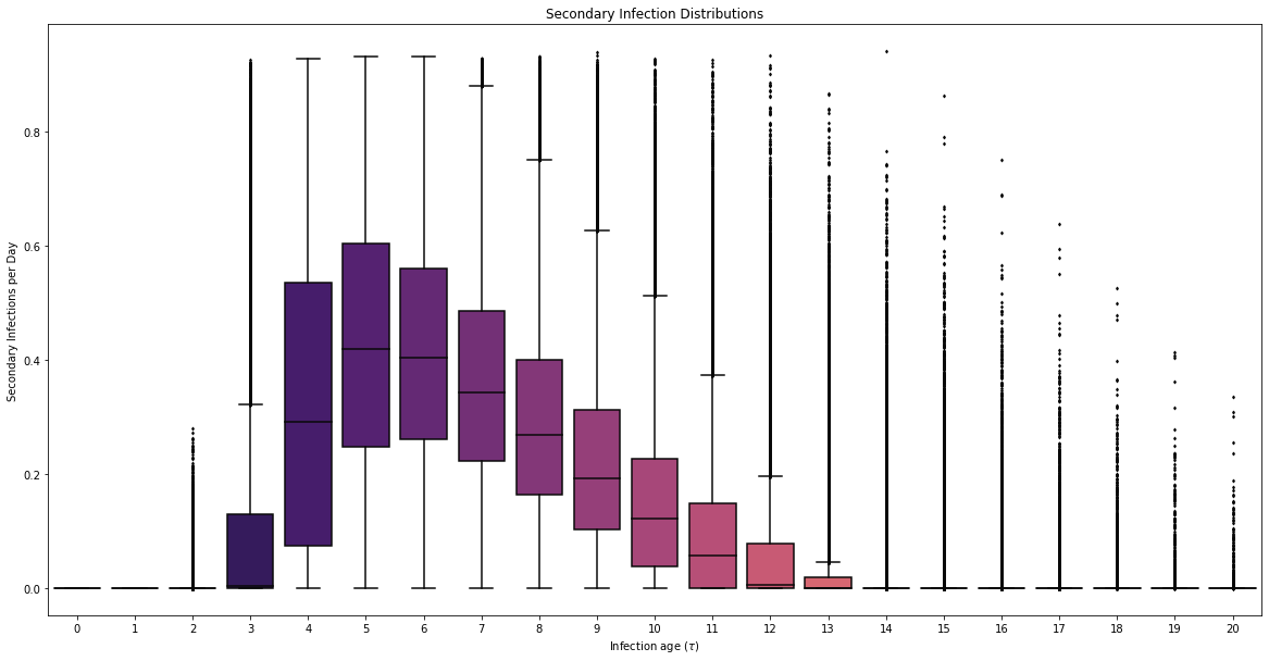
Individual Infectiousness
Infection Age
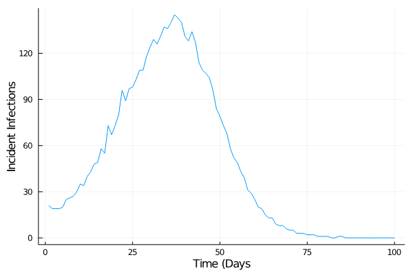
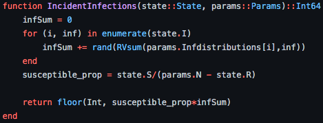
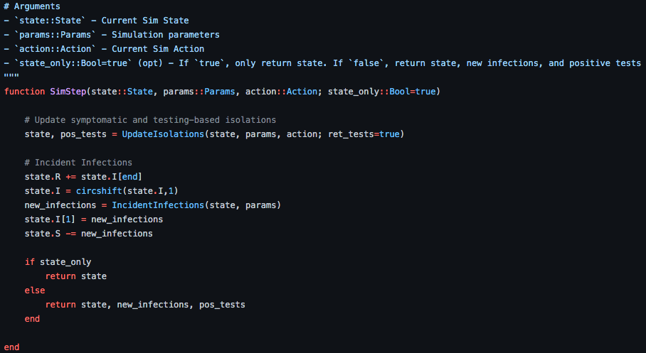
Incident Infections
\beta(\tau)
\tau
I
I(t) = \int_0^\infty I(t-\tau)\beta(\tau)d\tau
\beta(\tau)
Need
Test sensitivity is secondary to frequency and turnaround time for COVID-19 surveillance
Larremore et al.
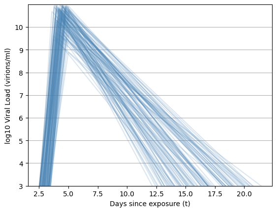
\beta(\tau) \propto \log_{10}(\text{viral load})
Viral load represented by piecewise-linear hinge function
(t_0, 3)
(t_{\text{peak}}, V_{\text{peak}})
(t_f,6)
t_0 \sim \mathcal{U}[2.5,3.5]
t_\text{peak} - t_0 \sim 0.2 + \text{Gamma}(1.8)
V_\text{peak} \sim \mathcal{U}[7,11]
t_f - t_\text{peak} \sim \mathcal{U}[5,10]
Test sensitivity is secondary to frequency and turnaround time for COVID-19 surveillance
Larremore et al.
Viral load represented by piecewise-linear hinge function
(t_0, 3)
(t_{\text{peak}}, V_{\text{peak}})
(t_f,6)
t_0 \sim \mathcal{U}[2.5,3.5]
t_\text{peak} - t_0 \sim 0.2 + \text{Gamma}(1.8)
V_\text{peak} \sim \mathcal{U}[7,11]
t_f - t_\text{peak} \sim \mathcal{U}[5,10]
Parametric Model Fitting
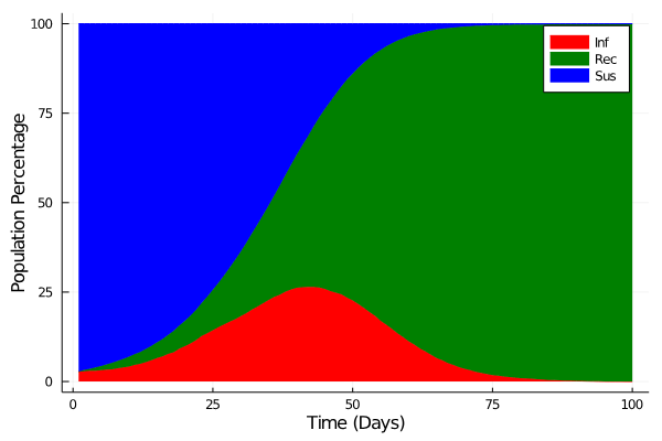
SIR Model
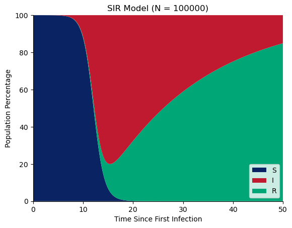
\dot{S} = -\beta I S \\
\dot{I} = \beta I S - \alpha I \\
\dot{R} = \alpha I
Susceptible
Infectious
Recovered
SEIR Model
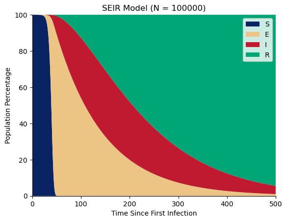
\dot{S} = -\beta I S \\
\dot{E} = \beta I S - \gamma E \\
\dot{I} = \gamma E - \alpha I \\
\dot{R} = \alpha I
Susceptible
Infectious
Recovered
Exposed

\dot{S} = -\beta I S \\
\dot{E} = \beta I S - \gamma E \\
\dot{I} = \gamma E - \alpha I \\
\dot{R} = \alpha I
\dot{S} = -\beta I S \\
\dot{I} = \beta I S - \alpha I \\
\dot{R} = \alpha I
\alpha \leftarrow \alpha + \delta T
\gamma \leftarrow \gamma + \epsilon T
\dot{S} = -\beta I S \\
\dot{I} = \beta I S - (\alpha + \delta T) I \\
\dot{R} = (\alpha + \delta T) I
\dot{S} = -\beta I S \\
\dot{E} = \beta I S - (\gamma + \epsilon T) E \\
\dot{I} = (\gamma + \epsilon T) E - \alpha I \\
\dot{R} = \alpha I
POMDP Formulation
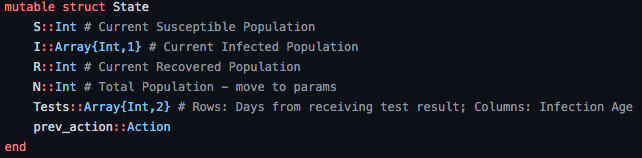
- Susceptible Population Count
- Infected Population Count
- Recovered Population Count
- Positive tests that are to be distributed
- Action taken on previous time step
\mathcal{S}
- Proportion of population tested
\mathcal{A}
- Quantity of positive tests
\mathcal{O}
\mathcal{R}
-\left\{c_I \left(\frac{1}{N}\sum_{i=1}^{H}I_i\right)^2 + c_T T^2 + c_{TR}(T_k - T_{k-1})^2\right\}
\mathcal{T}
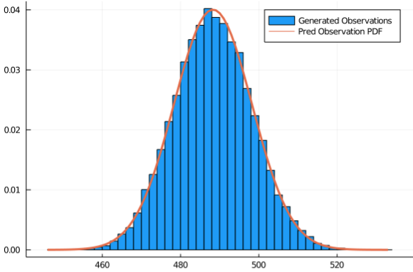
\mathcal{Z}
Positive test if viral load > LOD
\mathcal{Z}
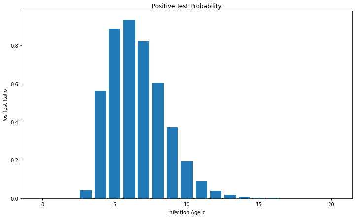
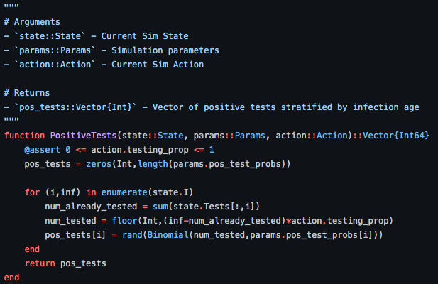
T_{pos,\tau} \sim \text{Bin}(n_\tau,p_\tau)
- tested infectious population
p_\tau
n_\tau
- probability of testing positive
\mathcal{Z}
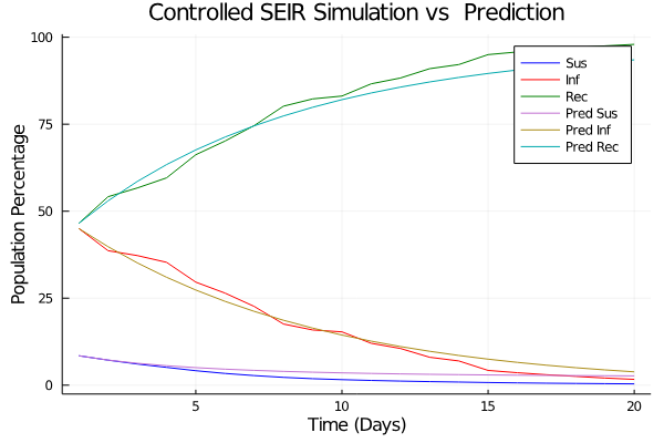
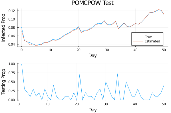
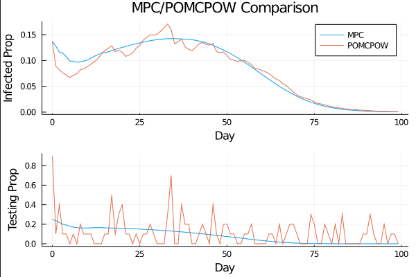
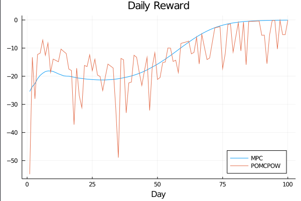
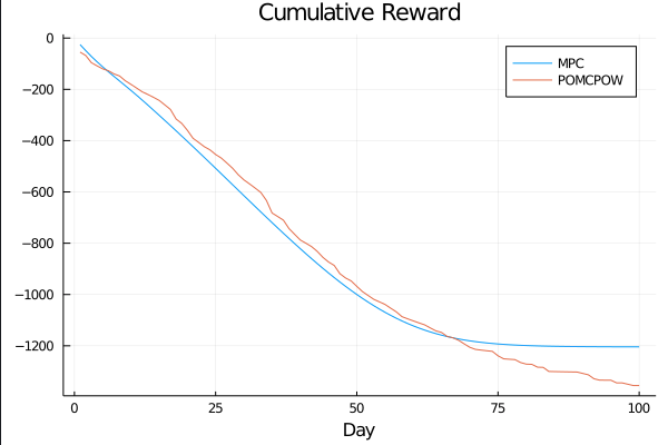
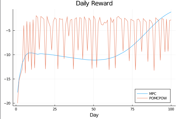
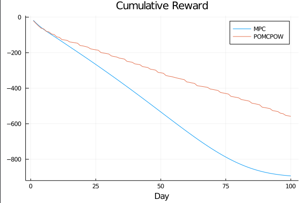
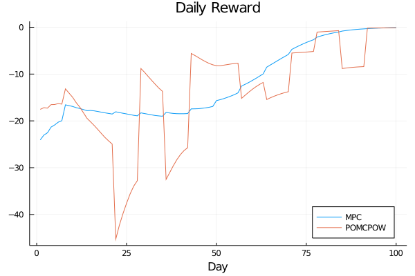
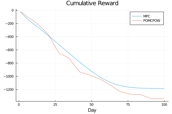
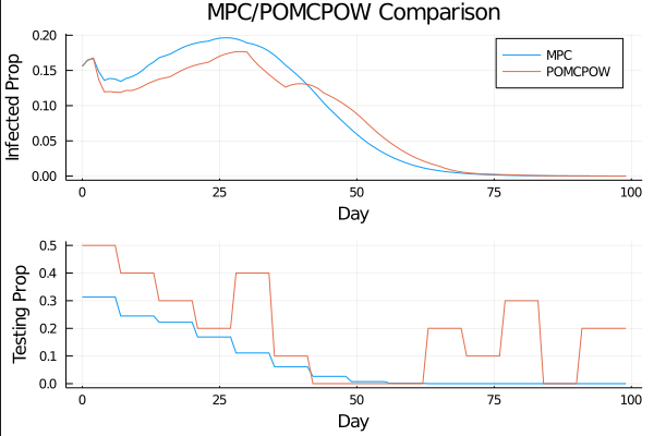
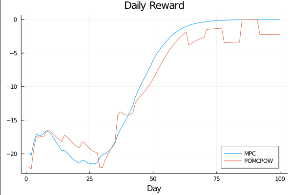
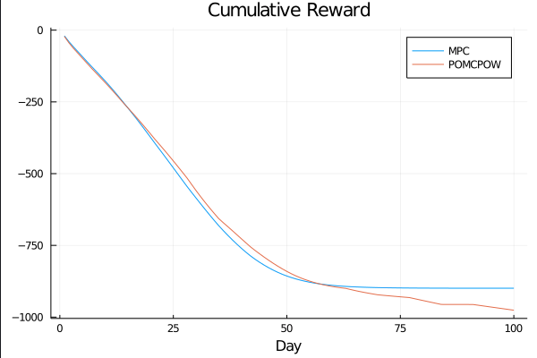
Controlled Model Results
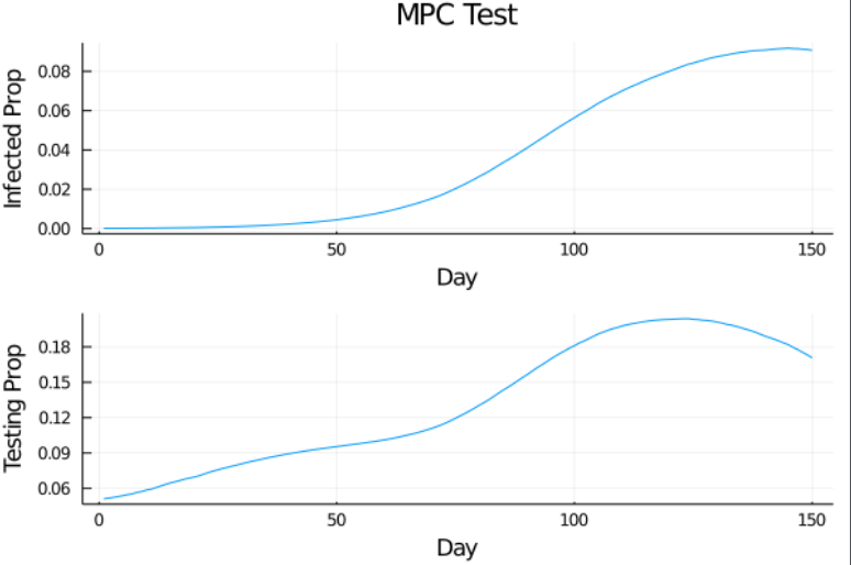
c_I = 100.0 \\
c_T = 1.0 \\
c_{TR} = 50.0
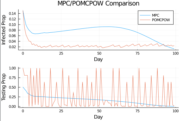
c_I = 100.0 \\
c_T = 1.0 \\
c_{TR} = 10.0
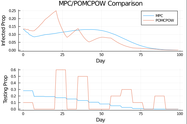
c_I = 100.0 \\
c_T = 1.0 \\
c_{TR} = 40.0
c_I = 100.0 \\
c_T = 1.0 \\
c_{TR} = 10.0
Future Plans
MPC with certainty equivalence works too well
- Unimodal belief
- Quadratic cost
- Continuous action space
- High frequency - low amplitude effect of noise
Possible avenue to more interesting results:
Introduce second viral strain
- Hopefully yields bimodal belief
- State space dimensionality almost doubled
Copy of Covid POMDP
By Zachary Sunberg


