
Breaking the Curse of Dimensionality in Decision-Making for Autonomous Systems
Assistant Professor Zachary Sunberg
University of Colorado Boulder
September 6th, 2024

Autonomous Decision and Control Laboratory

-
Algorithmic Contributions
- Scalable algorithms for partially observable Markov decision processes (POMDPs)
- Motion planning with safety guarantees
- Game theoretic algorithms
-
Theoretical Contributions
- Particle POMDP approximation bounds
-
Applications
- Space Domain Awareness
- Autonomous Driving
- Autonomous Aerial Scientific Missions
- Search and Rescue
- Space Exploration
- Ecology
-
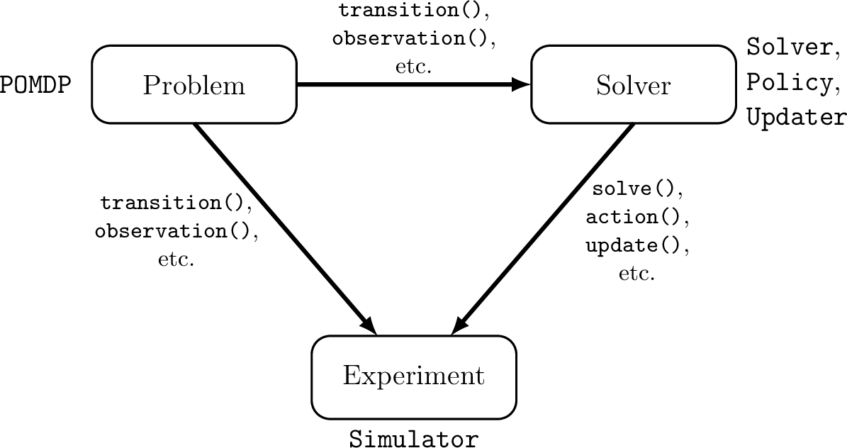
Open Source Software
- POMDPs.jl Julia ecosystem

PI: Prof. Zachary Sunberg

PhD Students


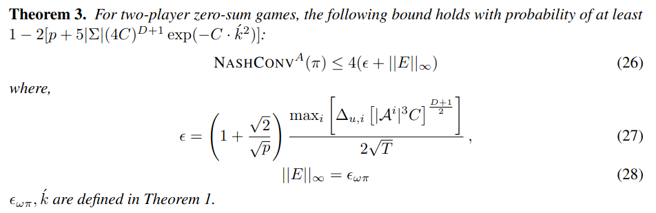
Postdoc

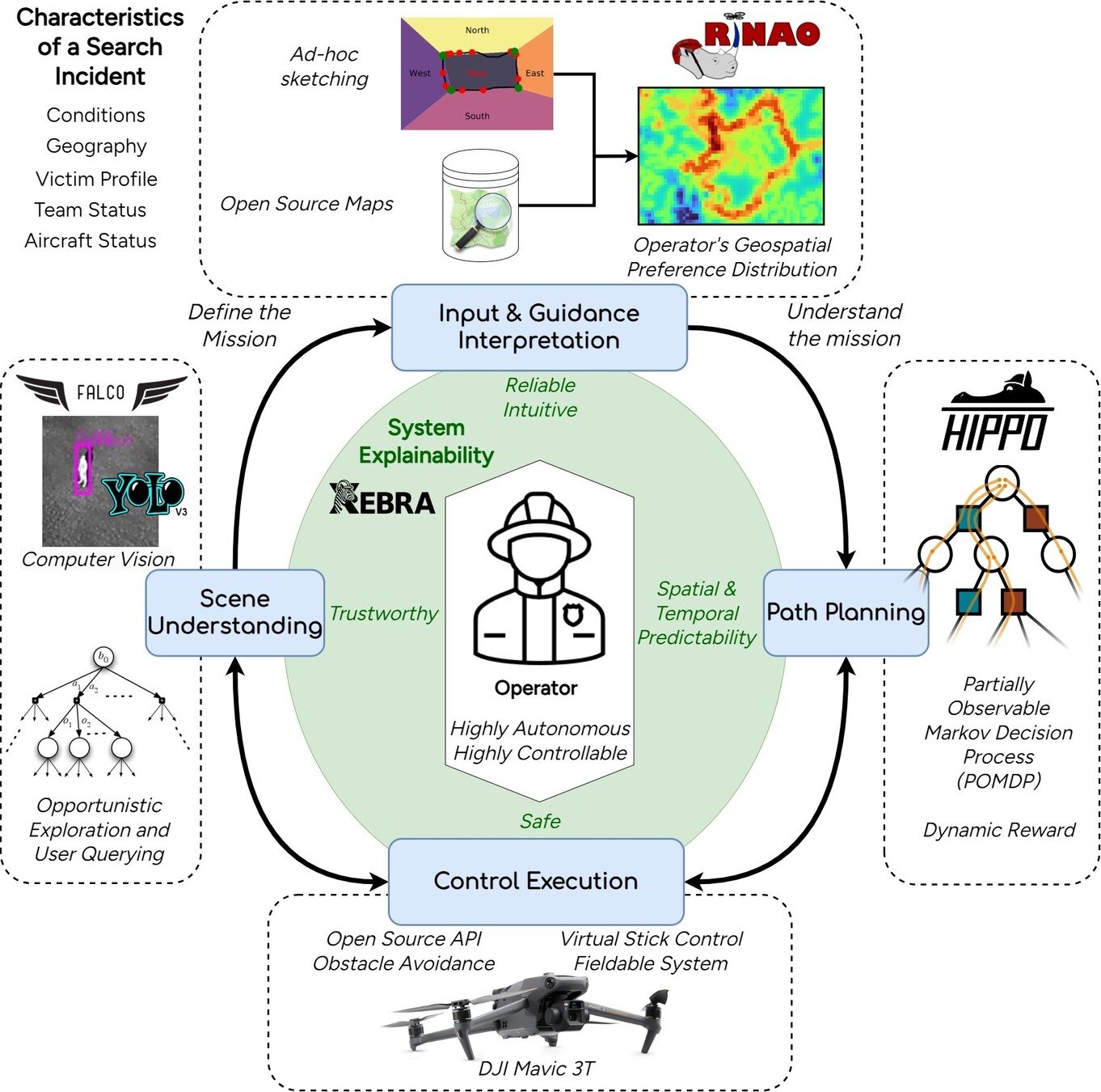
The ADCL creates autonomy that is safe and efficient despite uncertainty
Two Objectives for Autonomy
EFFICIENCY
SAFETY
Minimize resource use
(especially time)
Minimize the risk of harm to oneself and others
Safety often opposes Efficiency
Example 1: Autonomous Driving
Tweet by Nitin Gupta
29 April 2018
https://twitter.com/nitguptaa/status/990683818825736192
Example 1:
Autonomous Driving
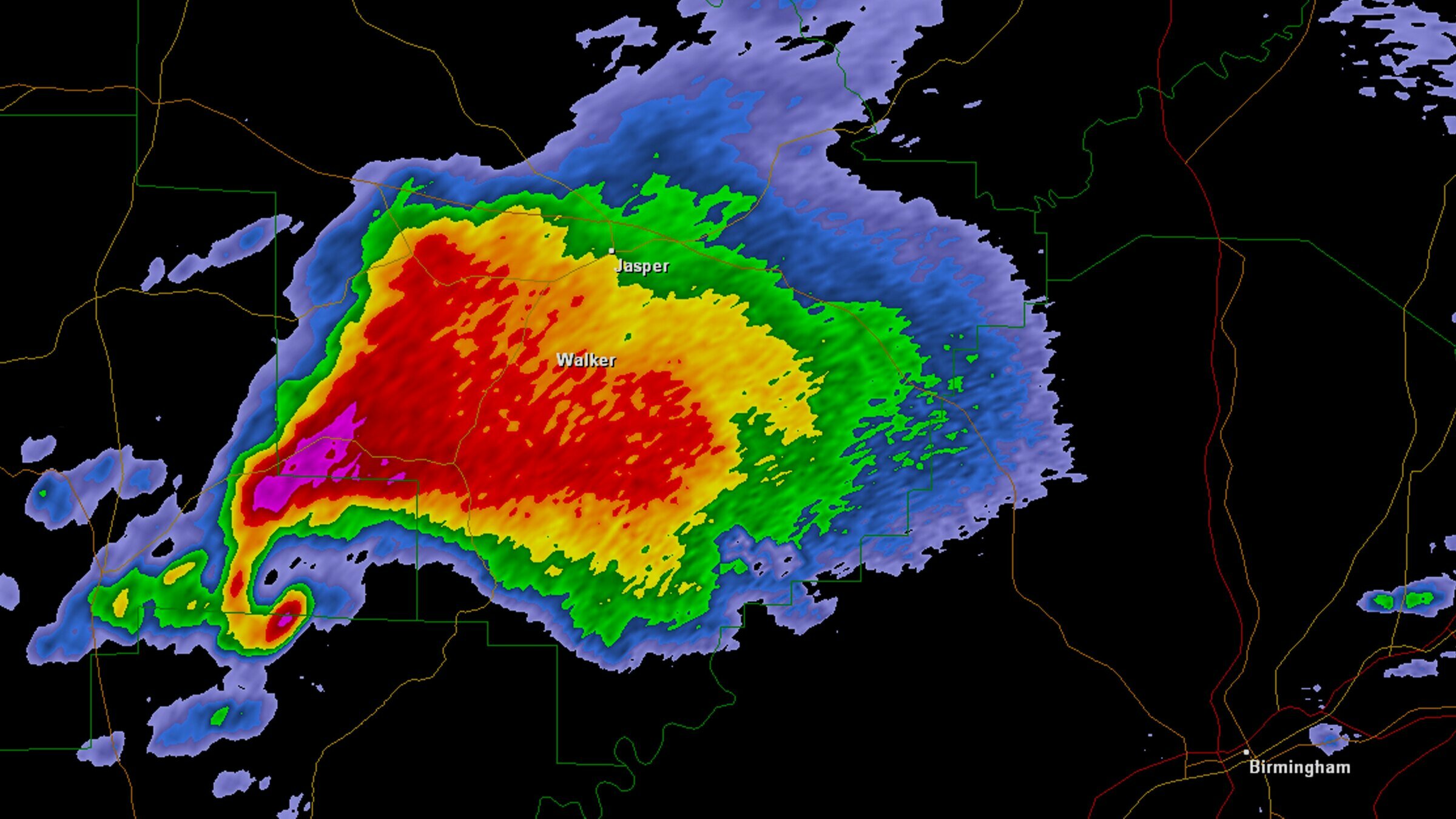
Example 2: Tornados
Video: Eric Frew
Example 2: Tornados
Video: Eric Frew
Example 2: Tornados
Video: Eric Frew
Example 2: Tornados

Example 3: Search and Rescue

What do they have in common?
Driving: what are the other road users going to do?
Tornado Forecasting: what is going on in the storm?
Search and Rescue: where is the lost person?
All are sequential decision-making problems with uncertainty!
All can be modeled as a POMDP (with a very large state and observation spaces).

Outline
- The Promise and Curse of POMDPs
- Breaking the Curse
- Applications
- Multiple Agents
Part I: The Promise and Curse of POMDPs
Types of Uncertainty
Aleatory
Epistemic (Static)
Epistemic (Dynamic)


Interaction
MDP
RL
POMDP
Game
Markov Decision Process (MDP)
- \(\mathcal{S}\) - State space
- \(T:\mathcal{S}\times \mathcal{A} \times\mathcal{S} \to \mathbb{R}\) - Transition probability distribution
- \(\mathcal{A}\) - Action space
- \(R:\mathcal{S}\times \mathcal{A} \to \mathbb{R}\) - Reward

Aleatory
\([x, y, z,\;\; \phi, \theta, \psi,\;\; u, v, w,\;\; p,q,r]\)
\(\mathcal{S} = \mathbb{R}^{12}\)
\(\mathcal{S} = \mathbb{R}^{12} \times \mathbb{R}^\infty\)
\[\underset{\pi:\, \mathcal{S} \to \mathcal{A}}{\text{maximize}} \quad \text{E}\left[ \sum_{t=0}^\infty R(s_t, a_t) \right]\]
Reinforcement Learning
- \(\mathcal{S}\) - State space
- \(T:\mathcal{S}\times \mathcal{A} \times\mathcal{S} \to \mathbb{R}\) - Transition probability distribution
- \(\mathcal{A}\) - Action space
- \(R:\mathcal{S}\times \mathcal{A} \to \mathbb{R}\) - Reward
Aleatory
Epistemic (Static)
\([x, y, z,\;\; \phi, \theta, \psi,\;\; u, v, w,\;\; p,q,r]\)
\(\mathcal{S} = \mathbb{R}^{12}\)
\(\mathcal{S} = \mathbb{R}^{12} \times \mathbb{R}^\infty\)
Partially Observable Markov Decision Process (POMDP)

- \(\mathcal{S}\) - State space
- \(T:\mathcal{S}\times \mathcal{A} \times\mathcal{S} \to \mathbb{R}\) - Transition probability distribution
- \(\mathcal{A}\) - Action space
- \(R:\mathcal{S}\times \mathcal{A} \to \mathbb{R}\) - Reward
- \(\mathcal{O}\) - Observation space
- \(Z:\mathcal{S} \times \mathcal{A}\times \mathcal{S} \times \mathcal{O} \to \mathbb{R}\) - Observation probability distribution
Aleatory
Epistemic (Static)
Epistemic (Dynamic)
\([x, y, z,\;\; \phi, \theta, \psi,\;\; u, v, w,\;\; p,q,r]\)
\(\mathcal{S} = \mathbb{R}^{12}\)
\(\mathcal{S} = \mathbb{R}^{12} \times \mathbb{R}^\infty\)
\begin{aligned}
& \mathcal{S} = \mathbb{Z} \quad \quad \quad ~~ \mathcal{O} = \mathbb{R} \\
& s' = s+a \quad \quad o \sim \mathcal{N}(s, |s-10|) \\
& \mathcal{A} = \{-10, -1, 0, 1, 10\} \\
& R(s, a) = \begin{cases}
100 & \text{ if } a = 0, s = 0 \\
-100 & \text{ if } a = 0, s \neq 0 \\
-1 & \text{ otherwise}
\end{cases} & \\
\end{aligned}

State
Timestep
Accurate Observations
Goal: \(a=0\) at \(s=0\)
Optimal Policy
Localize
\(a=0\)
POMDP Example: Light-Dark
Solving a POMDP
Environment
Belief Updater
Planner
\(a = +10\)

True State
\(s = 7\)
Observation \(o = -0.21\)

\(b\)
\[b_t(s) = P\left(s_t = s \mid b_0, a_0, o_1 \ldots a_{t-1}, o_{t}\right)\]
\[ = P\left(s_t = s \mid b_{t-1}, a_{t-1}, o_{t}\right)\]
\(Q(b, a)\)
\(O(|\mathcal{S}|^2)\)
Online Tree Search in MDPs

Time
Estimate \(Q(s, a)\) based on children
Bayesian Belief Updates
Environment
Belief Updater
Policy/Planner
\(b\)
\(a\)
\[b_t(s) = P\left(s_t = s \mid b_0, a_0, o_1 \ldots a_{t-1}, o_{t}\right)\]
True State
\(s = 7\)
Observation \(o = -0.21\)
\(O(|S|^2)\)
\[ = P\left(s_t = s \mid b_{t-1}, a_{t-1}, o_{t}\right)\]
Curse of History in POMDPs
Environment
Policy/Planner
\(a\)
True State
\(s = 7\)
Observation \(o = -0.21\)
Optimal planners need to consider the entire history
\(h_t = (b_0, a_0, o_1, a_1, o_2 \ldots a_{t-1}, o_{t})\)
A POMDP is an MDP on the Belief Space
POMDP \((S, A, T, R, O, Z)\) is equivalent to MDP \((S', A', T', R')\)
- \(S' = \Delta(S)\)
- \(A' = A\)
- \(T'\) defined by belief updates (\(T\) and \(Z\))
- \(R'(b, a) = \underset{s \sim b}{E}[R(s, a)]\)
One new continuous state dimension for each state in \(S\)!
Why are POMDPs difficult?
- Curse of History
- Curse of dimensionality
- State space
- Observation space
- Action space
Tree size: \(O\left(\left(|A||O|\right)^D\right)\)
POMDP (decision problem) is PSPACE Complete
Curse of Dimensionality
\(d\) dimensions, \(k\) segments \(\,\rightarrow \, |S| = k^d\)


1 dimension
e.g. \(s = x \in S = \{1,2,3,4,5\}\)
\(|S| = 5\)
2 dimensions
e.g. \(s = (x,y) \in S = \{1,2,3,4,5\}^2\)
\(|S| = 25\)
3 dimensions
e.g. \(s = (x,y,x_h) \in S = \{1,2,3,4,5\}^3\)
\(|S| = 125\)
(Discretize each dimension into 5 segments)

\(x\)
\(y\)
\(x_h\)

Part II: Breaking the Curse
Integration
Find \(\underset{s\sim b}{E}[f(s)]\)
\[=\sum_{s \in S} f(s) b(s)\]
Monte Carlo Integration
\(Q_N \equiv \frac{1}{N} \sum_{i=1}^N f(s_i)\)
\(s_i \sim b\) i.i.d.
\(\text{Var}(Q_N) = \text{Var}\left(\frac{1}{N} \sum_{i=1}^N f(s_i)\right)\)
\(= \frac{1}{N^2} \sum_{i=1}^N\text{Var}\left(f(s_i)\right)\)
\(= \frac{1}{N} \text{Var}\left(f(s_i)\right)\)
\[P(|Q_N - E[f(s_i)]| \geq \epsilon) \leq \frac{\text{Var}(f(s_i))}{N \epsilon^2}\]
(Bienayme)
(Chebyshev)
Curse of dimensionality!
Particle Filter POMDP Approximation
\[b(s) \approx \sum_{i=1}^N \delta_{s}(s_i)\; w_i\]
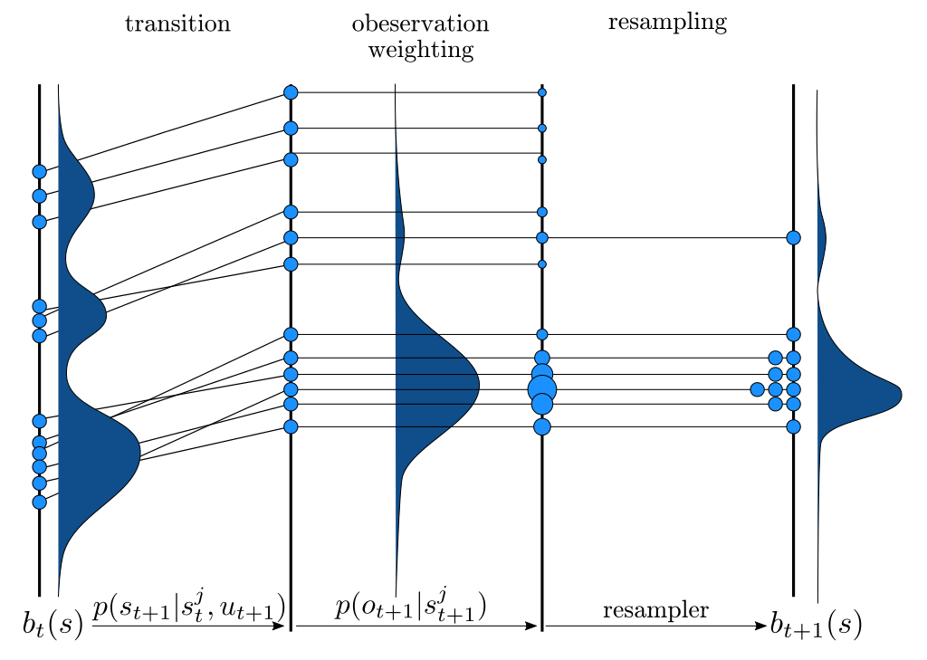

[Sunberg and Kochenderfer, ICAPS 2018, T-ITS 2022]
How do we prove convergence?
POMDP Assumptions for Proofs
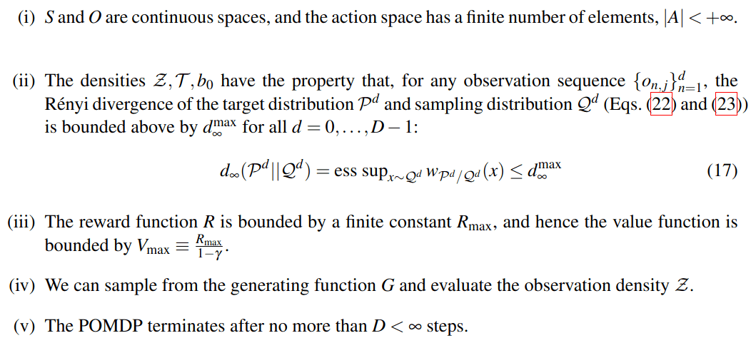

Continuous \(S\), \(O\); Discrete \(A\)
No Dirac-delta observation densities
Bounded Reward
Generative model for \(T\); Explicit model for \(Z\)
Finite Horizon
Only reasonable beliefs
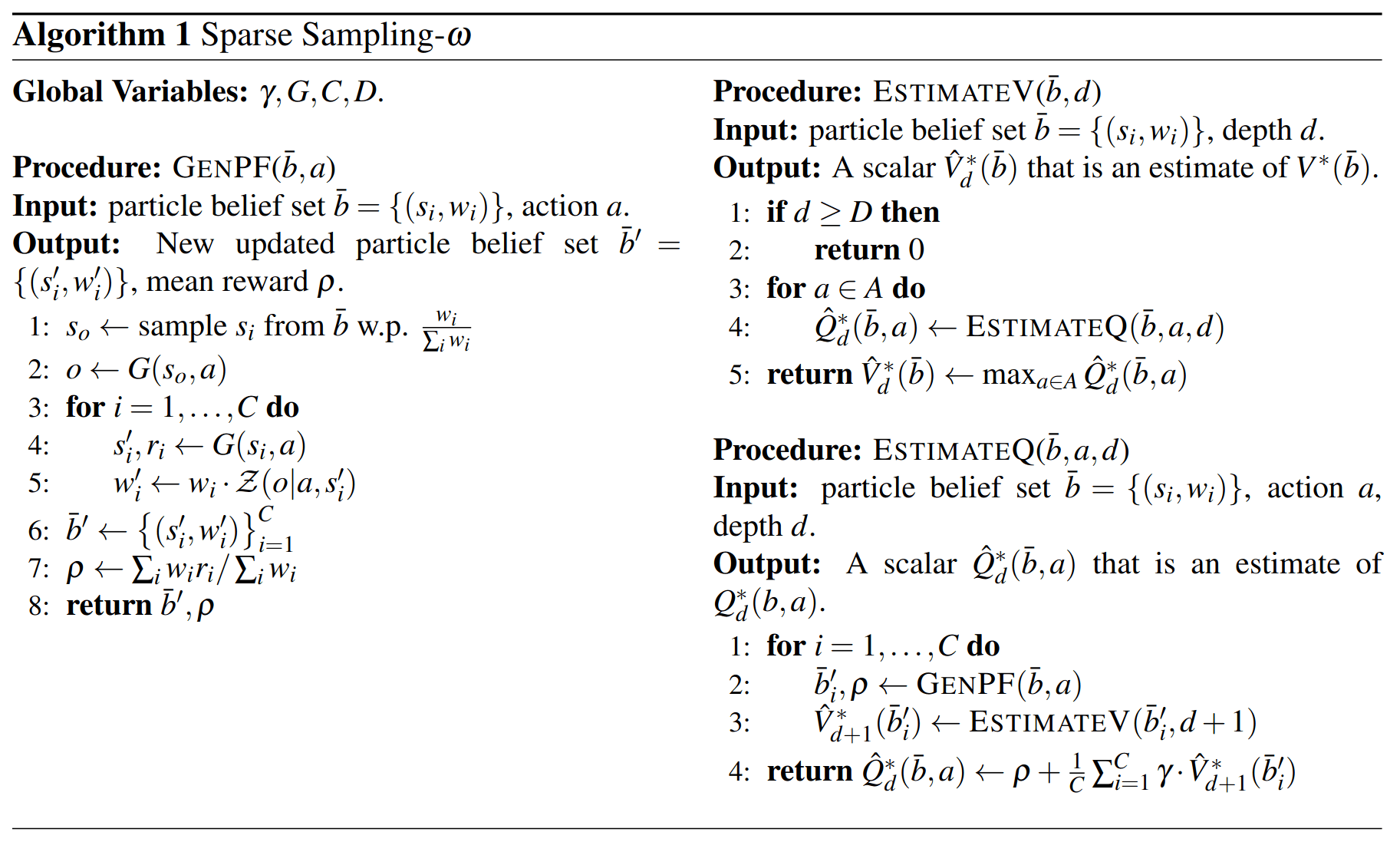
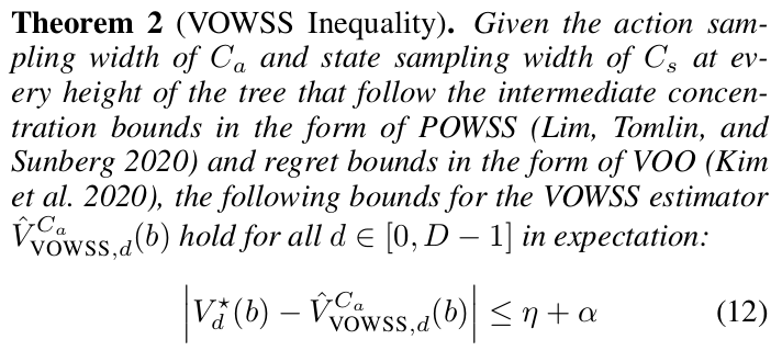
Sparse Sampling-\(\omega\)

Key 1: Self Normalized Infinite Renyi Divergence Concentation
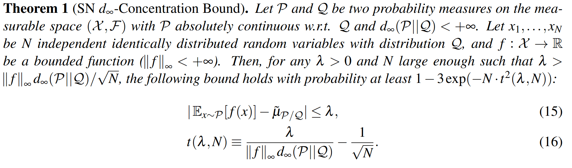
\(\mathcal{P}\): state distribution conditioned on observations (belief)
\(\mathcal{Q}\): marginal state distribution (proposal)
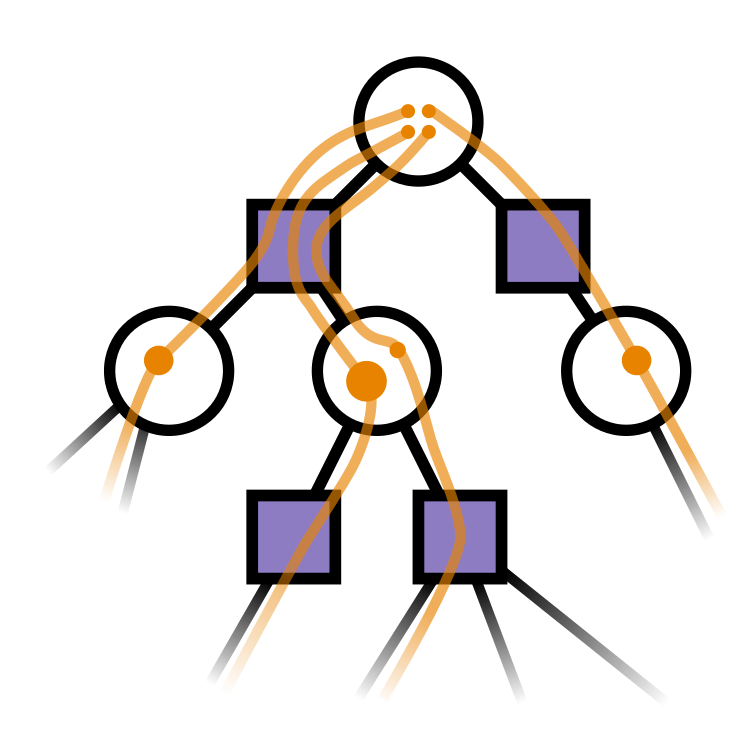
Key 2: Sparse Sampling
Expand for all actions (\(\left|\mathcal{A}\right| = 2\) in this case)
...
Expand for all \(\left|\mathcal{S}\right|\) states
\(C=3\) states
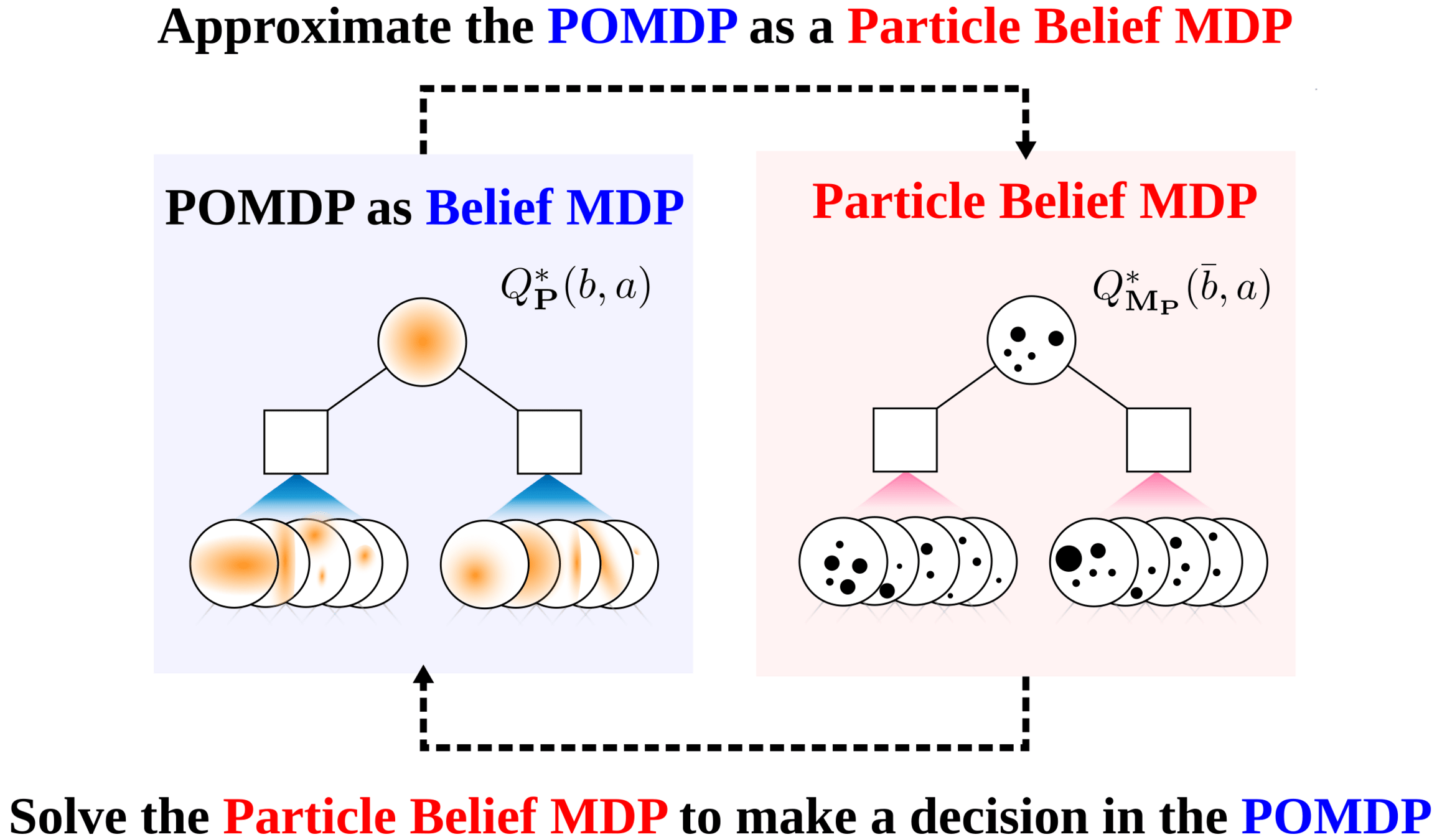
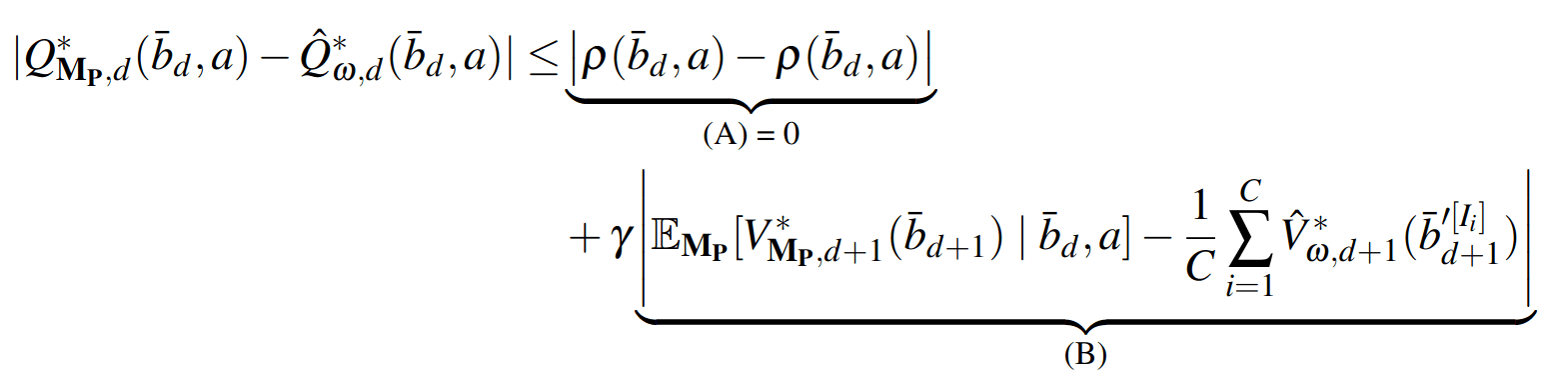
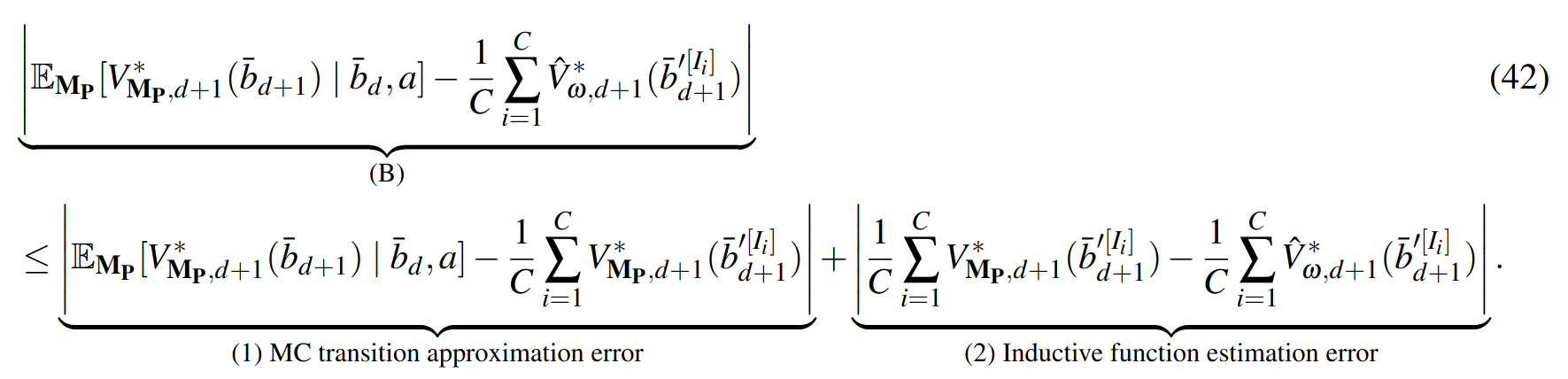
SS-\(\omega\) is close to Belief MDP
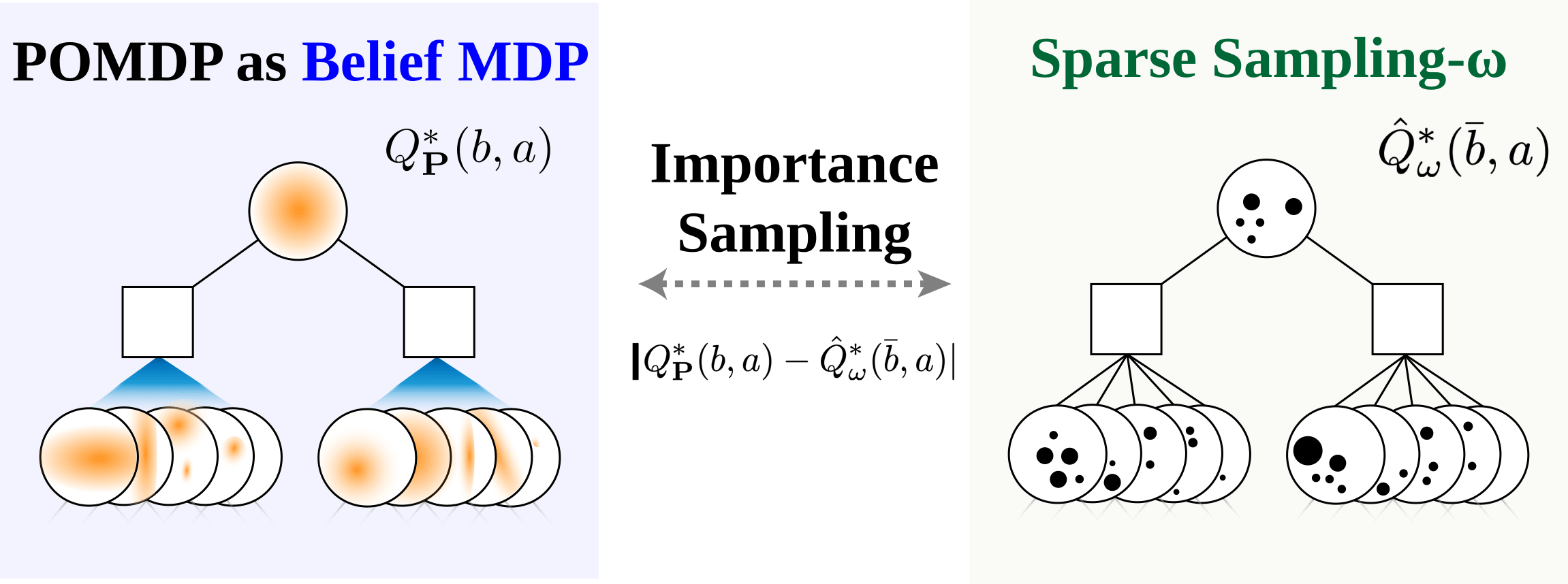
SS-\(\omega\) close to Particle Belief MDP (in terms of Q)

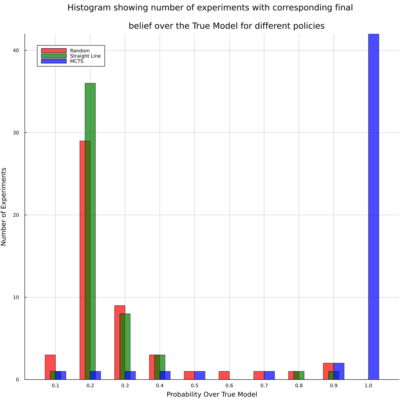
PF Approximation Accuracy
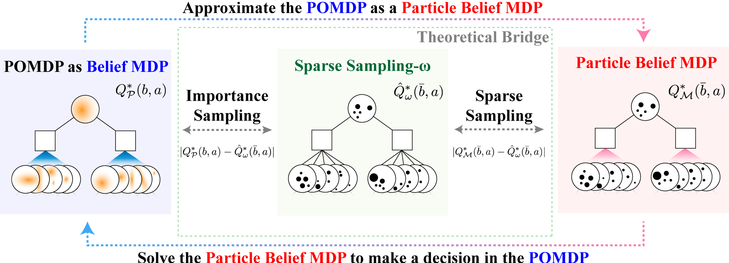
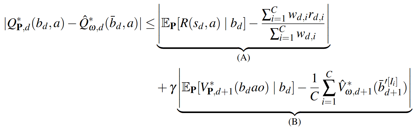
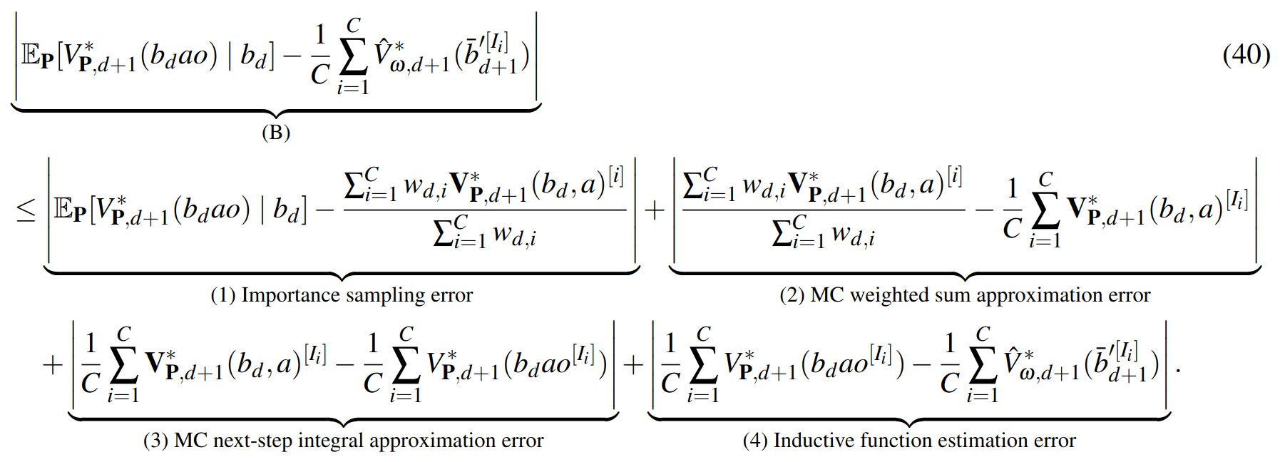
\[|Q_{\mathbf{P}}^*(b,a) - Q_{\mathbf{M}_{\mathbf{P}}}^*(\bar{b},a)| \leq \epsilon \quad \text{w.p. } 1-\delta\]
For any \(\epsilon>0\) and \(\delta>0\), if \(C\) (number of particles) is high enough,
[Lim, Becker, Kochenderfer, Tomlin, & Sunberg, JAIR 2023]
No direct dependence on \(|\mathcal{S}|\) or \(|\mathcal{O}|\)!

Particle belief planning suboptimality
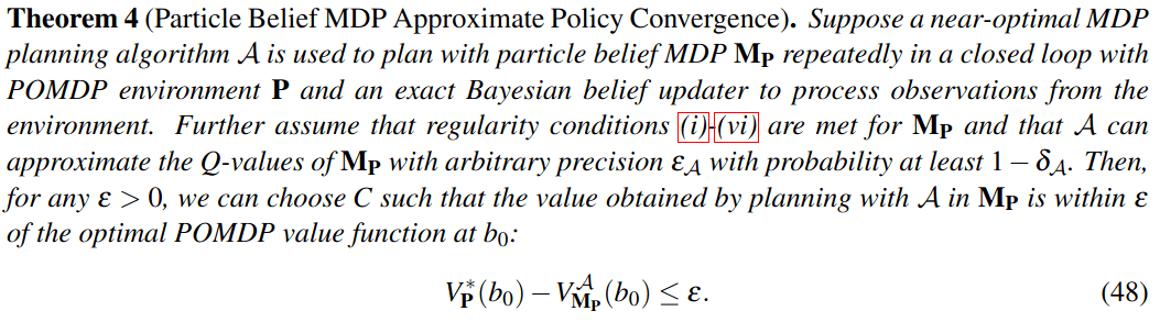
\(C\) is too large for any direct safety guarantees. But, in practice, works extremely well for improving efficiency.
[Lim, Becker, Kochenderfer, Tomlin, & Sunberg, JAIR 2023]
Why are POMDPs difficult?
- Curse of History
- Curse of dimensionality
- State space
- Observation space
- Action space

Tree size: \(O\left(\left(|A|C\right)^D\right)\)
Solve simplified surrogate problem for policy deep in the tree
[Lim, Tomlin, and Sunberg, 2021]
Easy MDP to POMDP Extension
Part III: Applications

Example 1: Autonomous Driving
POMDP Formulation
\(s=\left(x, y, \dot{x}, \left\{(x_c,y_c,\dot{x}_c,l_c,\theta_c)\right\}_{c=1}^{n}\right)\)
\(o=\left\{(x_c,y_c,\dot{x}_c,l_c)\right\}_{c=1}^{n}\)
\(a = (\ddot{x}, \dot{y})\), \(\ddot{x} \in \{0, \pm 1 \text{ m/s}^2\}\), \(\dot{y} \in \{0, \pm 0.67 \text{ m/s}\}\)
R(s, a, s') = \text{in\_goal}(s') - \lambda \left(\text{any\_hard\_brakes}(s, s') + \text{any\_too\_slow}(s')\right)

Ego external state
External states of other cars
Internal states of other cars
External states of other cars
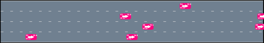
- Actions shielded (based only on external states) so they can never cause crashes
- Braking action always available
Efficiency
Safety
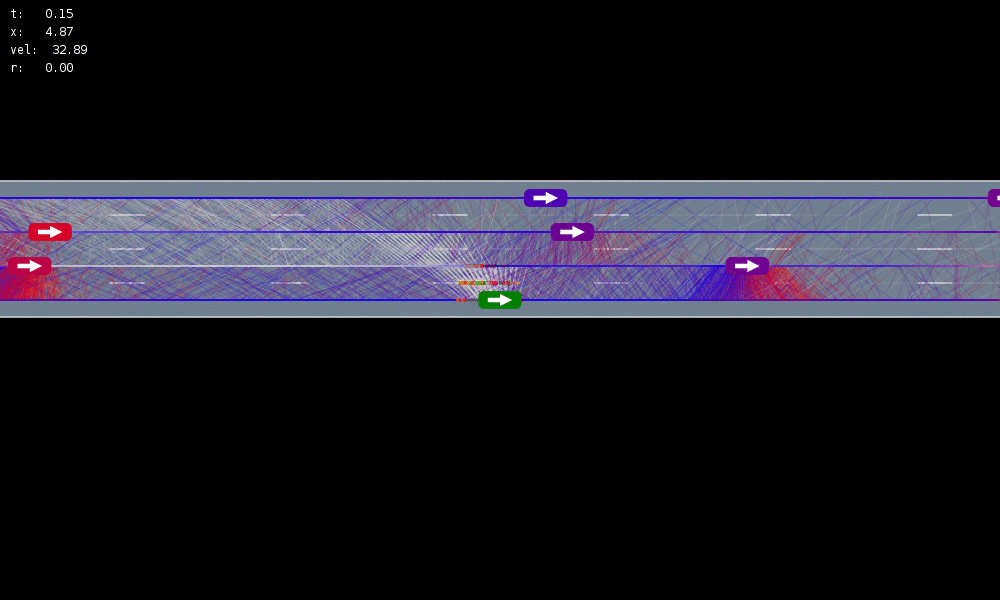


MDP trained on normal drivers


MDP trained on all drivers
Omniscient
POMCPOW (Ours)
Simulation results
[Sunberg & Kochenderfer, T-ITS 2023]
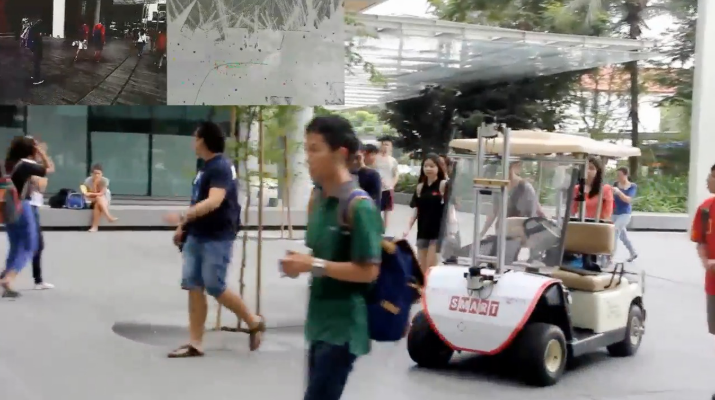
Navigation among Pedestrians
[Gupta, Hayes, & Sunberg, AAMAS 2022]
Previous solution: 1-D POMDP (92s avg)
Our solution (65s avg)
State:
- Vehicle physical state
- Human physical state
- Human intention

Conventional 1DOF POMDP
Multi-DOF POMDP
Pedestrian Navigation
[Gupta, Hayes, & Sunberg, AAMAS 2021]
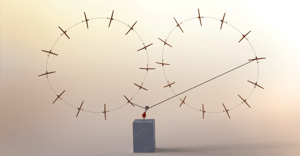
Meteorology
- State: (physical state of aircraft, which forecast is the truth)
- Action: (flight direction, drifter deploy)
- Reward: Terminal reward for correct weather prediction
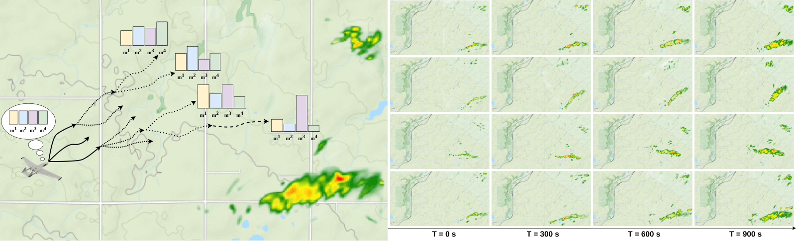
Example 2: Tornado Prediction
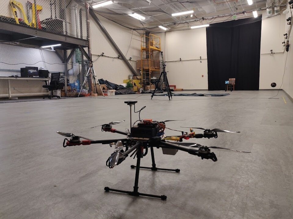
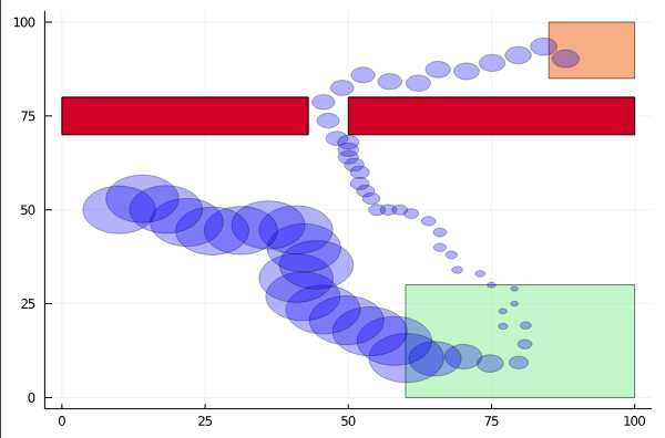
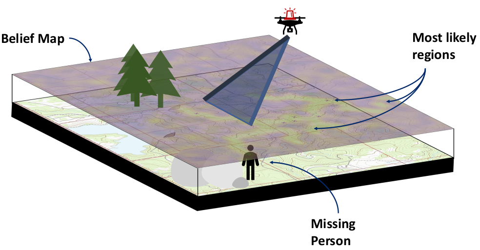
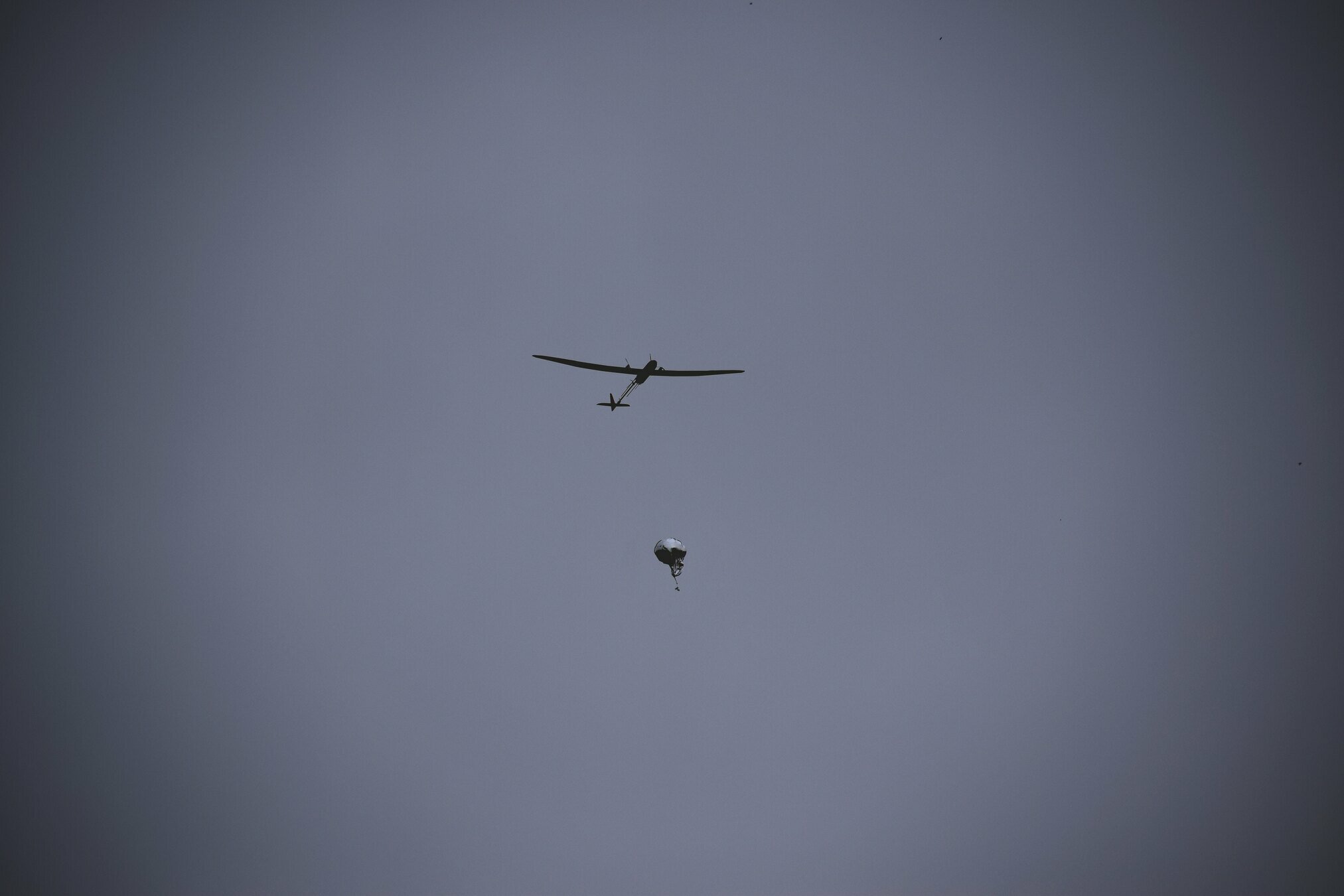
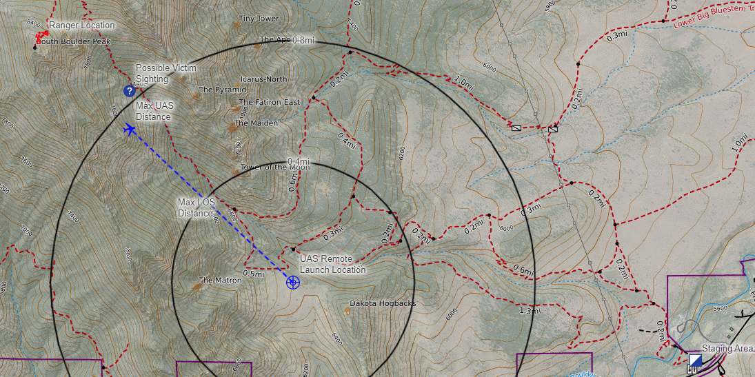
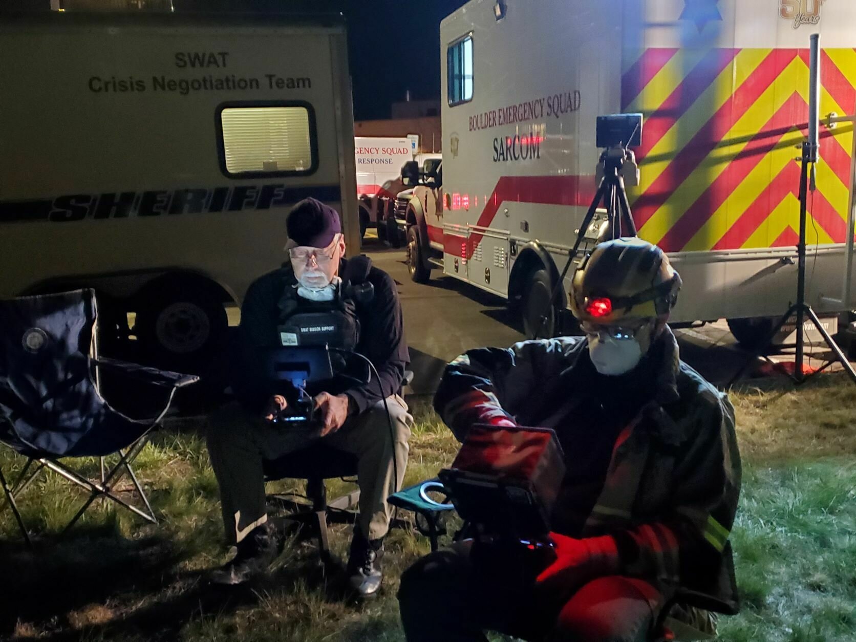
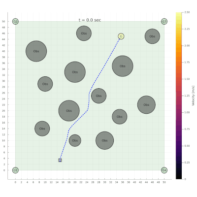
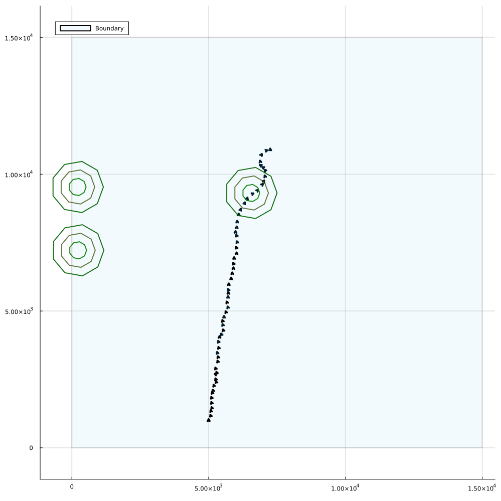
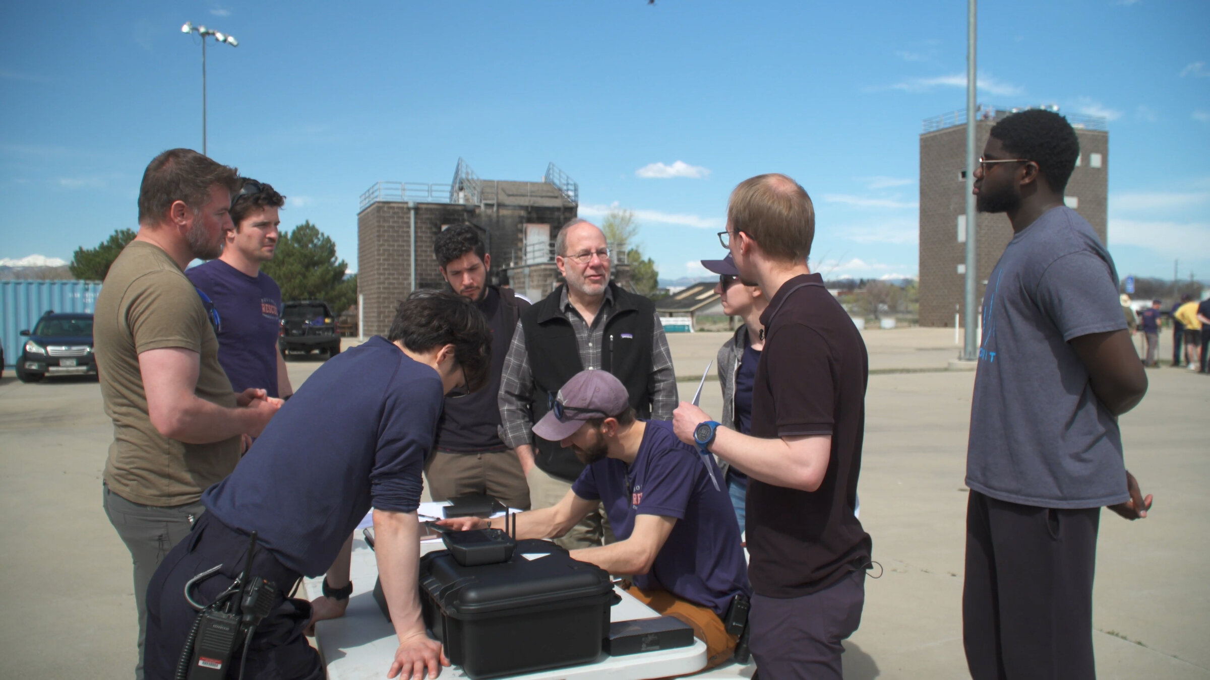
Drone Search and Rescue
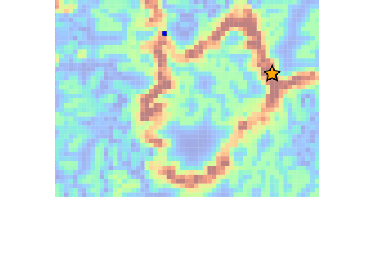
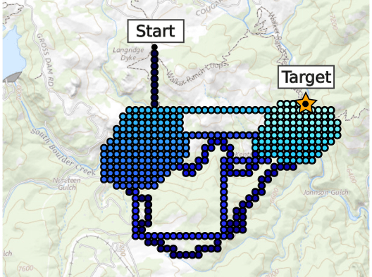

State:
- Location of Drone
- Location of Human
Baseline
Our POMDP Planner
[Ray, Laouar, Sunberg, & Ahmed, ICRA 2023]
Drone Search and Rescue

[Ray, Laouar, Sunberg, & Ahmed, ICRA 2023]
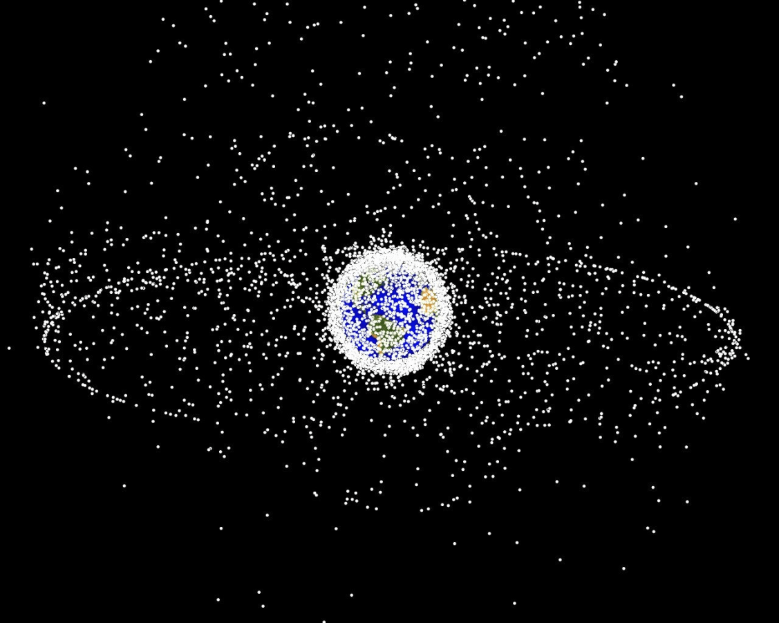
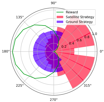
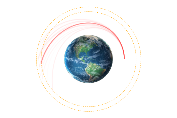
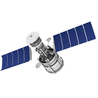
Space Domain Awareness

(Result for simplified dynamical system)
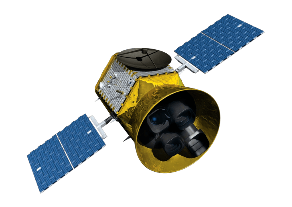
State:
- Position, velocity of object-of-interest
- Anomalies: navigation failure, suspicious maneuver, thruster failure, etc.
Innovation: Large language models allow analysts to quickly specify anomaly hypotheses
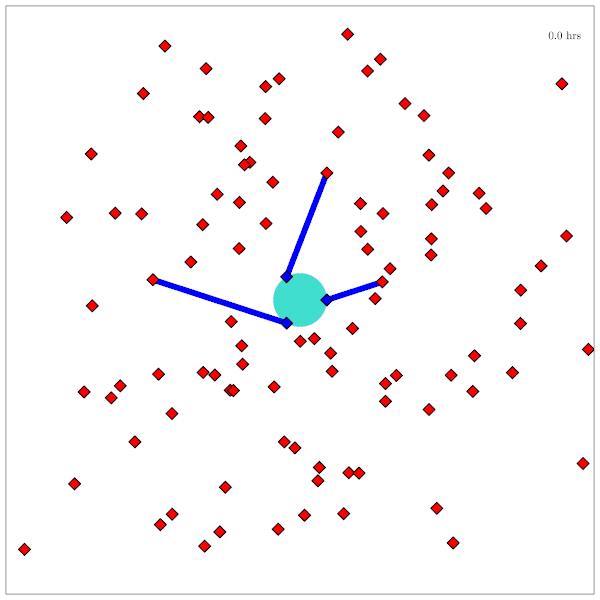
Catalog Maintenance Plan
Practical Safety Guarantees
Three Contributions
- Recursive constraints (solves "stochastic self-destruction")
- Undiscounted POMDP solutions for estimating probability
- Much faster motion planning with Gaussian uncertainty
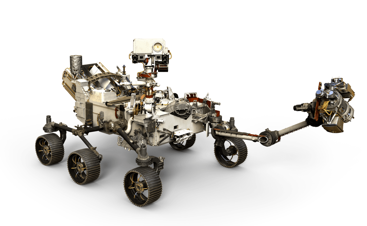

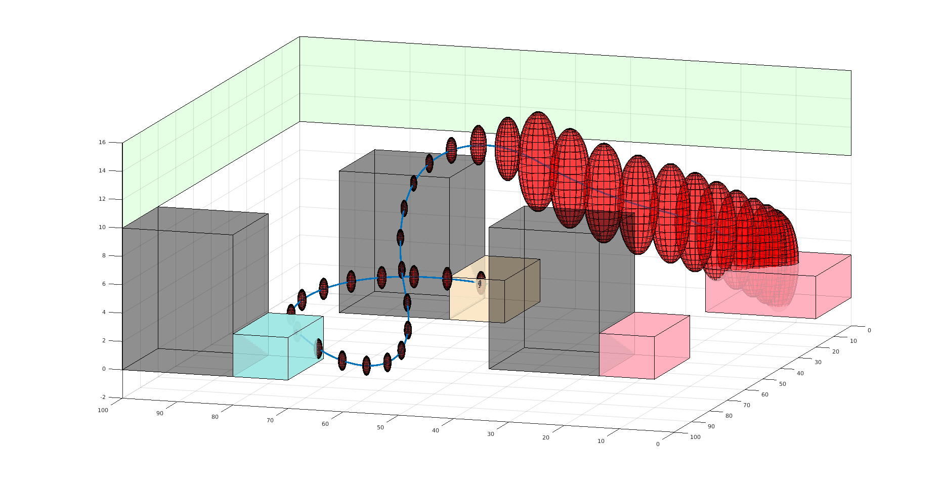
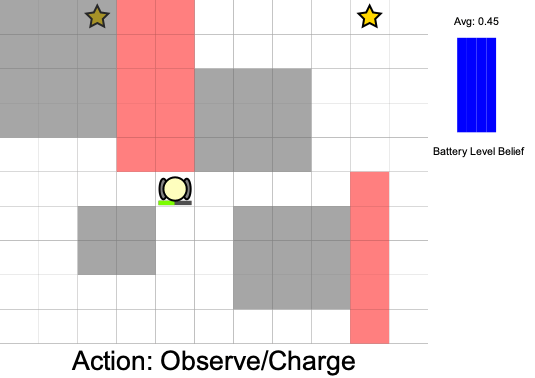
State:
- Position of rover
- Environment state: e.g. traversibility
- Internal status: e.g. battery, component health
[Ho et al., UAI 24], [Ho, Feather, Rossi, Sunberg, & Lahijanian, UAI 24], [Ho, Sunberg, & Lahijanian, ICRA 22]
Explainability: Reward Reconciliation

Calculate Outcomes
Calculate Weight Update
\( \frac{\epsilon - \alpha_a \cdot \Delta \mu_{h-a}}{\Delta\mu_{h-j} \cdot \Delta \mu_{h-a}} \Delta\mu_{h-j}\)
Estimate Weight with Update
\( \alpha[2]\)
\( \alpha[1]\)
\( a_{h}\) - optimal
\( a_{a}\) - optimal
\( \alpha_{h}\)
\( \alpha_{a}\)
\( R(s,a) = \alpha \cdot \boldsymbol{\phi}(s,a)\)
\(a_a\) outcomes: \(\mu_a\)
\(a_h\) outcomes: \(\mu_h\)
\(a_a\)
\(a_h\)
\( \hat{\alpha}_{h}\)
\(a_h\)
\(a_a\)
[Kraske, Saksena, Buczak, & Sunberg, ICAA 2024]
Part IV: Multiple Agents
Partially Observable Markov Decision Process (POMDP)
- \(\mathcal{S}\) - State space
- \(T:\mathcal{S}\times \mathcal{A} \times\mathcal{S} \to \mathbb{R}\) - Transition probability distribution
- \(\mathcal{A}\) - Action space
- \(R:\mathcal{S}\times \mathcal{A} \to \mathbb{R}\) - Reward
- \(\mathcal{O}\) - Observation space
- \(Z:\mathcal{S} \times \mathcal{A}\times \mathcal{S} \times \mathcal{O} \to \mathbb{R}\) - Observation probability distribution
Aleatory
Epistemic (Static)
Epistemic (Dynamic)
Partially Observable Stochastic Game (POSG)
Aleatory
Epistemic (Static)
Epistemic (Dynamic)
Interaction
- \(\mathcal{S}\) - State space
- \(T(s' \mid s, \bm{a})\) - Transition probability distribution
- \(\mathcal{A}^i, \, i \in 1..k\) - Action spaces
- \(R^i(s, \bm{a})\) - Reward function (cooperative, opposing, or somewhere in between)
- \(\mathcal{O}^i, \, i \in 1..k\) - Observation spaces
- \(Z(o^i \mid \bm{a}, s')\) - Observation probability distributions

Game Theory
Nash Equilibrium: All players play a best response.
Optimization Problem
(MDP or POMDP)
\(\text{maximize} \quad f(x)\)
Game
Player 1: \(U_1 (a_1, a_2)\)
Player 2: \(U_2 (a_1, a_2)\)
Collision
Example: Airborne Collision Avoidance
|
|
|
|
|
Player 1
Player 2
Up
Down
Up
Down
-6, -6
-1, 1
1, -1
-4, -4

Collision
Mixed Strategies
Nash Equilibrium \(\iff\) Zero Exploitability
\[\sum_i \max_{\pi_i'} U_i(\pi_i', \pi_{-i})\]
No Pure Nash Equilibrium!
Instead, there is a Mixed Nash where each player plays up or down with 50% probability.
If either player plays up or down more than 50% of the time, their strategy can be exploited.
Exploitability (zero sum):
Strategy (\(\pi_i\)): probability distribution over actions
|
|
|
|
|
Up
Down
Up
Down
-1, 1
1, -1
1, -1
-1, 1
Collision
Collision


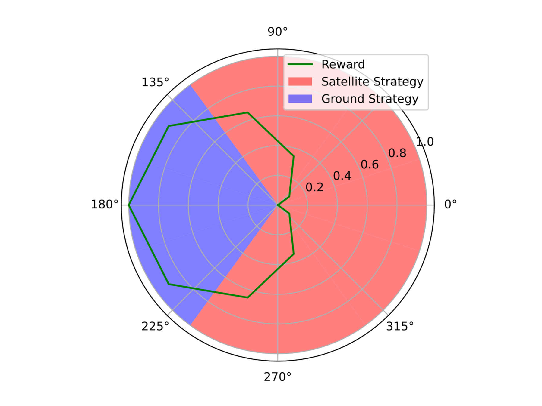
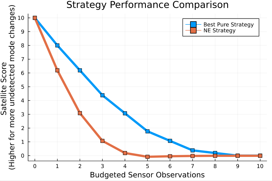
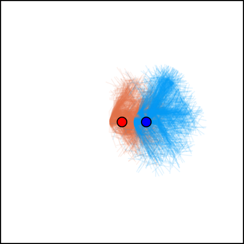
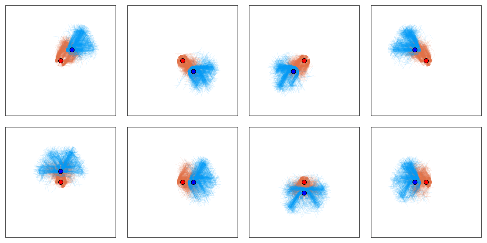
Space Domain Awareness Games
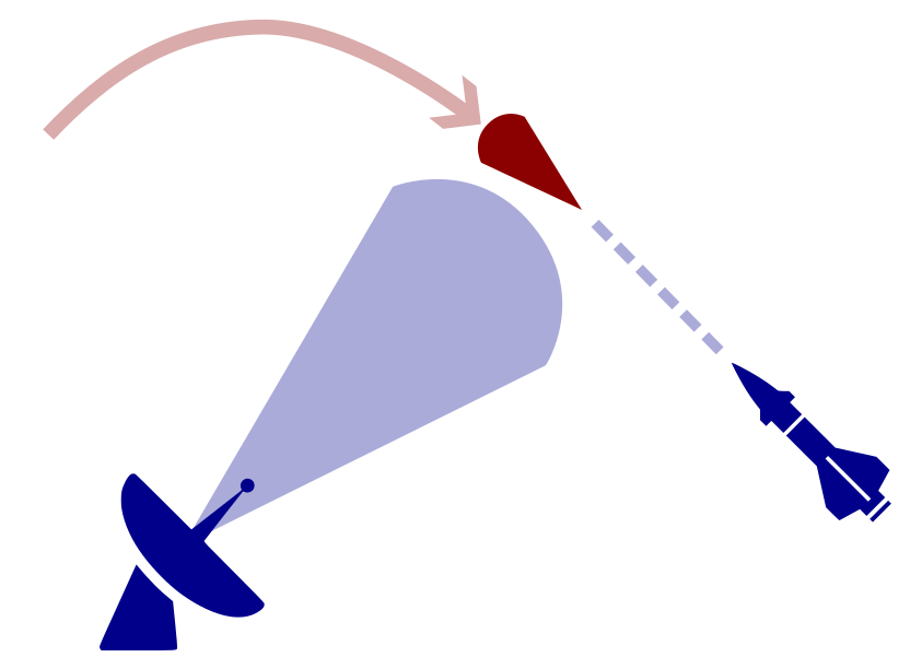
POSG Example: Missile Defense
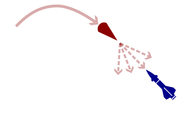
POMDP Solution:
- Assume a distribution for the missile's actions
- Update belief according to this distribution
- Use a POMDP planner to find the best defensive action
Nash equilibrium: All players play a best response to the other players
Fundamentally impossible for POMDP solvers to compute.
May include stochastic behavior (bluffing)
A shrewd missile operator will use different actions, invalidating our belief
Defending against Maneuverable Hypersonic Weapons: the Challenge
Ballistic
Maneuverable Hypersonic
- Sense
- Estimate
- Intercept
Every maneuver involves tradeoffs
- Energy
- Targets
- Intentions
Simplified SDA Game

1
2
...
...
...
...
...
...
...
\(N\)
[Becker & Sunberg, AMOS 2022]
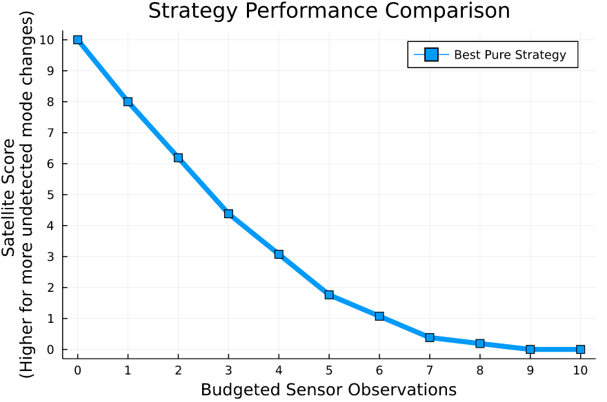
[Becker & Sunberg, AMOS 2022]
Counterfactual Regret Minimization Training
[Becker & Sunberg, AMOS 2022]
[Becker & Sunberg, AMOS 2022]
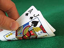
Finding a Nash Equilibrium: Poker
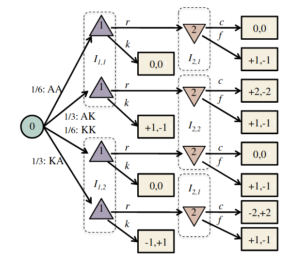
Image: Russel & Norvig, AI, a modern approach
P1: A
P1: K
P2: A
P2: A
P2: K
Tree Search Algorithms for POSGs
[Becker & Sunberg, NeurIPS 2024 (Under Review)]
Tree Search Algorithms for POSGs
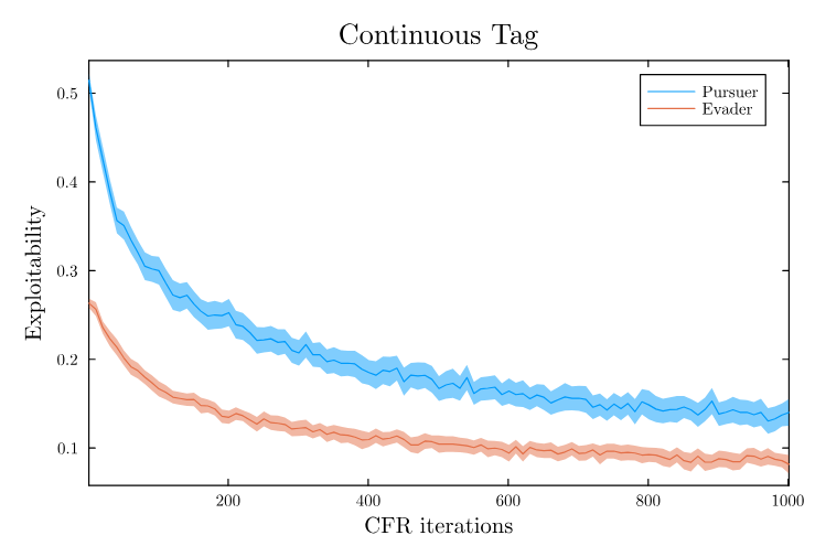
[Becker & Sunberg, NeurIPS 2024 (Under Review)]
Thank You!


Funding orgs: (all opinions are my own)


VADeR
Autonomous Decision and Control Laboratory
-
Algorithmic Contributions
- Scalable algorithms for partially observable Markov decision processes (POMDPs)
- Motion planning with safety guarantees
- Game theoretic algorithms
-
Theoretical Contributions
- Particle POMDP approximation bounds
-
Applications
- Space Domain Awareness
- Autonomous Driving
- Autonomous Aerial Scientific Missions
- Search and Rescue
- Space Exploration
- Ecology
-
Open Source Software
- POMDPs.jl Julia ecosystem
PI: Prof. Zachary Sunberg
PhD Students
Postdoc
Part V: Open Source Research Software
Good Examples
- Open AI Gym interface
- OMPL
- ROS
Challenges for POMDP Software
- There is a huge variety of
- Problems
- Continuous/Discrete
- Fully/Partially Observable
- Generative/Explicit
- Simple/Complex
- Solvers
- Online/Offline
- Alpha Vector/Graph/Tree
- Exact/Approximate
- Domain-specific heuristics
- Problems
- POMDPs are computationally difficult.
Explicit
Black Box
("Generative" in POMDP lit.)

\(s,a\)
\(s', o, r\)
Previous C++ framework: APPL
"At the moment, the three packages are independent. Maybe one day they will be merged in a single coherent framework."
Open Source Research Software
- Performant
- Flexible and Composable
- Free and Open
- Easy for a wide range of people to use (for homework)
- Easy for a wide range of people to understand
C++
Python, C++
Python, Matlab
Python, Matlab
Python, C++
2013

We love [Matlab, Lisp, Python, Ruby, Perl, Mathematica, and C]; they are wonderful and powerful. For the work we do — scientific computing, machine learning, data mining, large-scale linear algebra, distributed and parallel computing — each one is perfect for some aspects of the work and terrible for others. Each one is a trade-off.
We are greedy: we want more.
2012
POMDPs.jl - An interface for defining and solving MDPs and POMDPs in Julia

Mountain Car
partially_observable_mountaincar = QuickPOMDP(
    actions = [-1., 0., 1.],
    obstype = Float64,
    discount = 0.95,
    initialstate = ImplicitDistribution(rng -> (-0.2*rand(rng), 0.0)),
    isterminal = s -> s[1] > 0.5,

    gen = function (s, a, rng)
        x, v = s
        vp = clamp(v + a*0.001 + cos(3*x)*-0.0025, -0.07, 0.07)
        xp = x + vp
        if xp > 0.5
            r = 100.0
        else
            r = -1.0
        end
        return (sp=(xp, vp), r=r)
    end,

    observation = (a, sp) -> Normal(sp[1], 0.15)
)
using POMDPs
using QuickPOMDPs
using POMDPPolicies
using Compose
import Cairo
using POMDPGifs
import POMDPModelTools: Deterministic
mountaincar = QuickMDP(
function (s, a, rng)
x, v = s
vp = clamp(v + a*0.001 + cos(3*x)*-0.0025, -0.07, 0.07)
xp = x + vp
if xp > 0.5
r = 100.0
else
r = -1.0
end
return (sp=(xp, vp), r=r)
end,
actions = [-1., 0., 1.],
initialstate = Deterministic((-0.5, 0.0)),
discount = 0.95,
isterminal = s -> s[1] > 0.5,
render = function (step)
cx = step.s[1]
cy = 0.45*sin(3*cx)+0.5
car = (context(), circle(cx, cy+0.035, 0.035), fill("blue"))
track = (context(), line([(x, 0.45*sin(3*x)+0.5) for x in -1.2:0.01:0.6]), stroke("black"))
goal = (context(), star(0.5, 1.0, -0.035, 5), fill("gold"), stroke("black"))
bg = (context(), rectangle(), fill("white"))
ctx = context(0.7, 0.05, 0.6, 0.9, mirror=Mirror(0, 0, 0.5))
return compose(context(), (ctx, car, track, goal), bg)
end
)
energize = FunctionPolicy(s->s[2] < 0.0 ? -1.0 : 1.0)
makegif(mountaincar, energize; filename="out.gif", fps=20)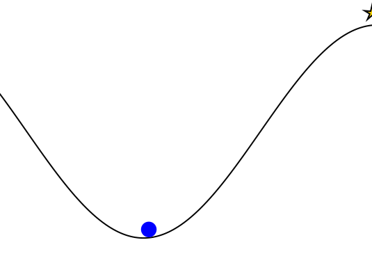


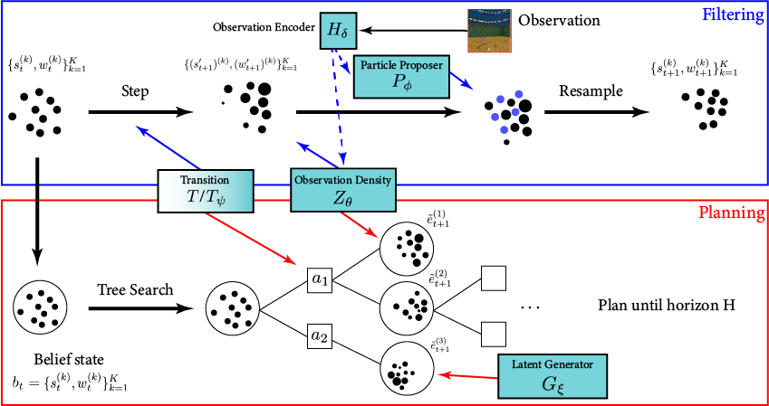
POMDP Planning with Learned Components
[Deglurkar, Lim, Sunberg, & Tomlin, 2023]
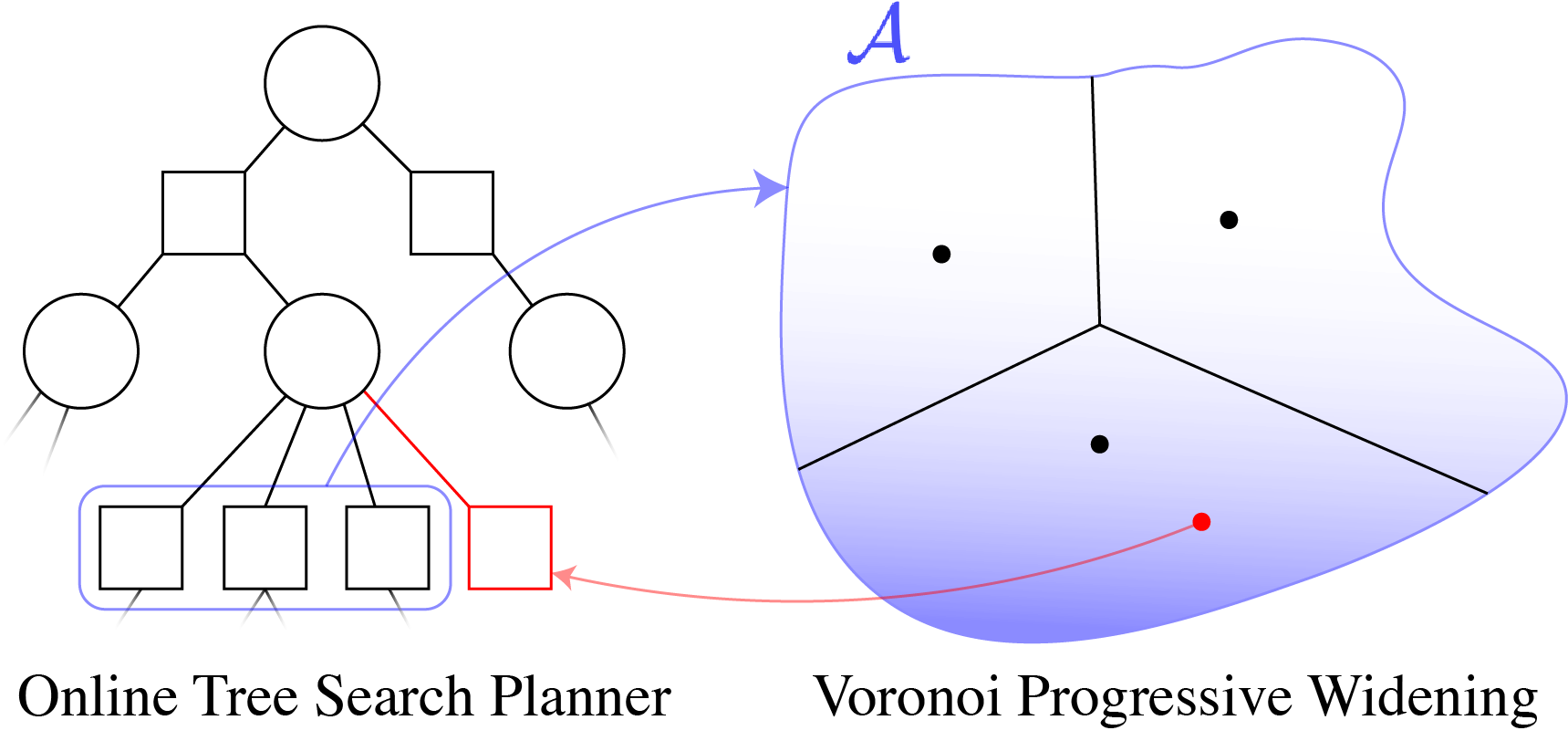
Continuous \(A\): BOMCP


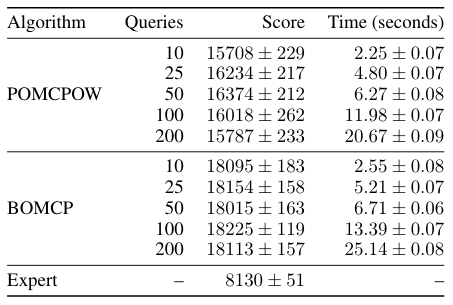
[Mern, Sunberg, et al. AAAI 2021]
Continuous \(A\): Voronoi Progressive Widening
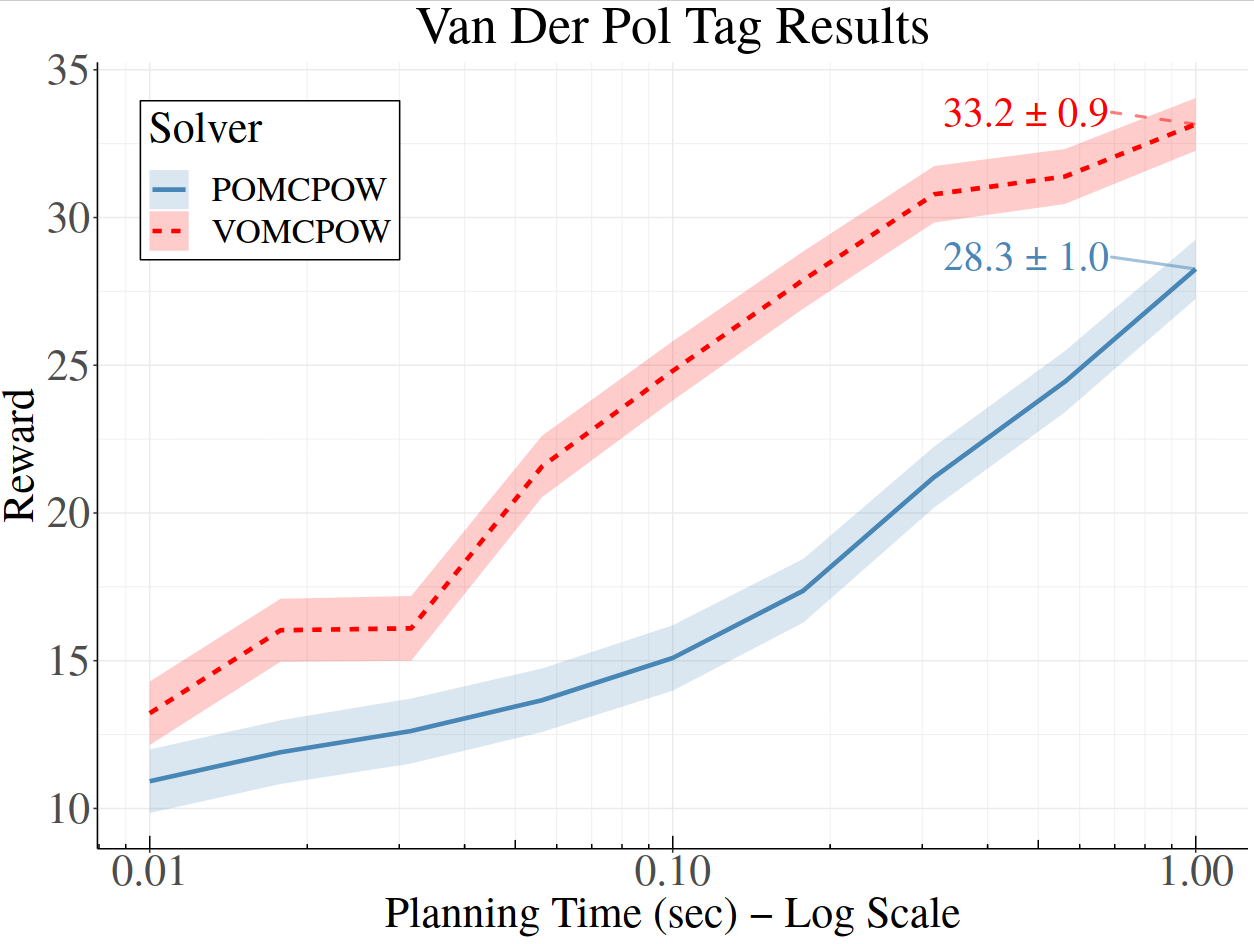
[Lim, Tomlin, & Sunberg CDC 2021]
Storm Science
Human Behavior Model: IDM and MOBIL
\ddot{x}_\text{IDM} = a \left[ 1 - \left( \frac{\dot{x}}{\dot{x}_0} \right)^{\delta} - \left(\frac{g^*(\dot{x}, \Delta \dot{x})}{g}\right)^2 \right]
g^*(\dot{x}, \Delta \dot{x}) = g_0 + T \dot{x} + \frac{\dot{x}\Delta \dot{x}}{2 \sqrt{a b}}

M. Treiber, et al., “Congested traffic states in empirical observations and microscopic simulations,” Physical Review E, vol. 62, no. 2 (2000).
A. Kesting, et al., “General lane-changing model MOBIL for car-following models,” Transportation Research Record, vol. 1999 (2007).
A. Kesting, et al., "Agents for Traffic Simulation." Multi-Agent Systems: Simulation and Applications. CRC Press (2009).


All drivers normal


Omniscient
Mean MPC
QMDP
POMCPOW
Reappointment Seminar
By Zachary Sunberg


