"Optimal Trajectories of Curvature-Constrained Motion in the Hamilton-Jacobi Formulation"
Authors: Ryo Takei & Richard Tsai (UCLA, 2013)
Presenter: William Pope
Motivation
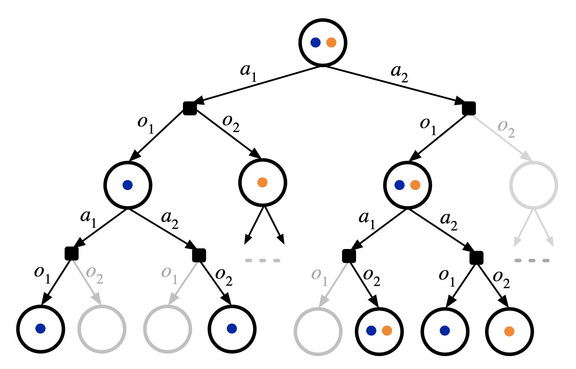
- Tree-based online (PO)MDP solvers use rollout simulations to initialize new nodes
- Reward is sparse in navigation scenarios, so need a good rollout policy to guide
- Value estimate must be generated quickly to build search tree online
- HJB provides on-demand optimal trajectories from any point in space, used for rollout in pedestrian navigation problem
Multi-Query Motion Planning
- Can use multi-query planning as policy for rollout simulations
- Single run of planner algorithm provides complete trajectories on-demand from any point in state space
- Common multi-query methods:
- Fast marching method (FMM)
- Probabilistic roadmaps (PRM)
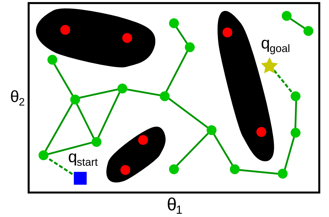
PRM
FMM
However: these methods don't work well for systems with differential constraints
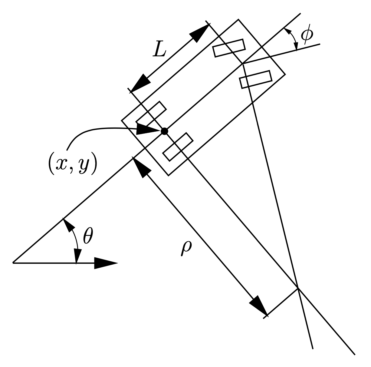
Curvature-Constrained Dynamics
- Simple nonlinear kinematic model used to approximate motion of a car
- Assumes instantaneous changes in speed and steering angle
\dot{x} = f(x,u) = \begin{bmatrix} \dot{x} \\ \dot{y} \\ \dot{\theta} \end{bmatrix} = \begin{bmatrix} u_{v} \cos{\theta} \\ u_{v} \sin{\theta} \\ u_{v}\frac{1}{l}\tan{u_{\phi}} \end{bmatrix}
u = \begin{bmatrix} u_{v} \\ u_{\phi} \end{bmatrix}
x = \begin{bmatrix} x \\ y \\ \theta \end{bmatrix}
Reeds-Shepp Curves
- For vehicle with car-like steering, shortest path between two states will always be a series of straight lines connected by minimum-radius curves, driven at max speed
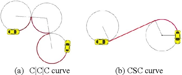
U_{opt} = \begin{Bmatrix} (\max(u_{v}), 0.0) & (\min(u_{v}), 0.0) \\ (\max(u_{v}), \max(u_{\phi}) & (\min(u_{v}), \max(u_{\phi}) \\ (\max(u_{v}), \min(u_{\phi}) & (\min(u_{v}), \min(u_{\phi}) \end{Bmatrix}
- So for first-order dynamics, continuous-time optimal action will always be 1 of 6:
Hamilton-Jacobi-Bellman Equation
- PDE for finding global optimal control of a system (Bellman, 1950s)
- Value function: minimum cost-to-go over given time interval
-
- C – cost rate function
- D – terminal value
V(x(t_{0}),t_{0}) = \min_{u}\{\int_{t_{0}}^{t_{f}} C(x(\tau),u(\tau)) d\tau + D(x(t_{f}))\}
V(x(t_{0}),t_{0}) = \min_{u}\{V(x(t_{0}+dt),t_{0}+dt) + \int_{t_{0}}^{t_{0}+dt} C(x(\tau),u(\tau)) d\tau\}
- Rewriting with dynamic programming principle:
Hamilton-Jacobi-Bellman Equation
- Applying Taylor series expansion to right side:
V(x(t),t) = \min_{u}\{V(x(t+dt),t+dt) + \int_{t}^{t+dt} C(...) d\tau\}
V(x(t),t) = \min_{u}\{V(x(t),t) + \frac{\partial V}{\partial t}dt + \frac{\partial V}{\partial x}dx + \int_{t}^{t+dt} C(...) d\tau\}
V(x(t),t) = V(x(t),t) + \frac{\partial V}{\partial t}dt + \min_{u}\{\frac{\partial V}{\partial x}\dot{x}dt + \int_{t}^{t+dt} C(...) d\tau\}
0 = \frac{\partial V}{\partial t} + \min_{u}\{\frac{\partial V}{\partial x}\dot{x} + \frac{1}{dt}\int_{t}^{t+dt} C(...) d\tau\}
0 = \frac{\partial V}{\partial t} + \min_{u}\{\frac{\partial V}{\partial x}f(x,u) + C(x,u) \}
- Hamilton-Jacobi-Bellman partial differential equation:
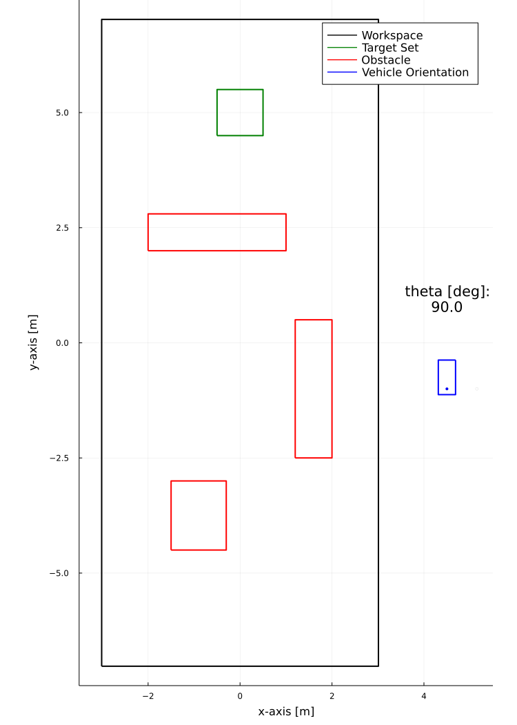
Solving HJB for Optimal Trajectories
- Offline:
- Given map of environment, discretize state space
- Assign known value to target set
- Solve PDE for value function V(x,y,θ) using finite difference method iterated over grid nodes
- Online:
- Use gradient descent to generate optimal path from current leaf node
- Simulate rollout using optimal path, return value to search tree
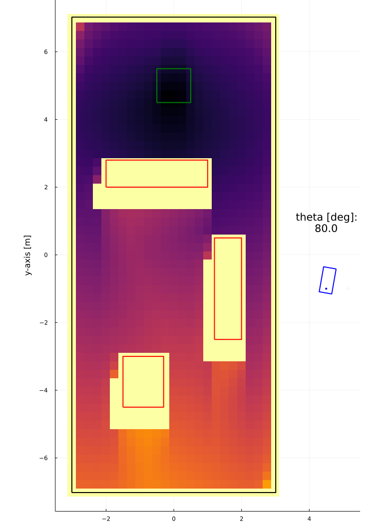
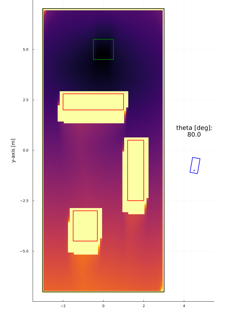
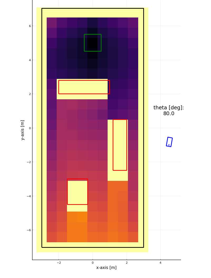
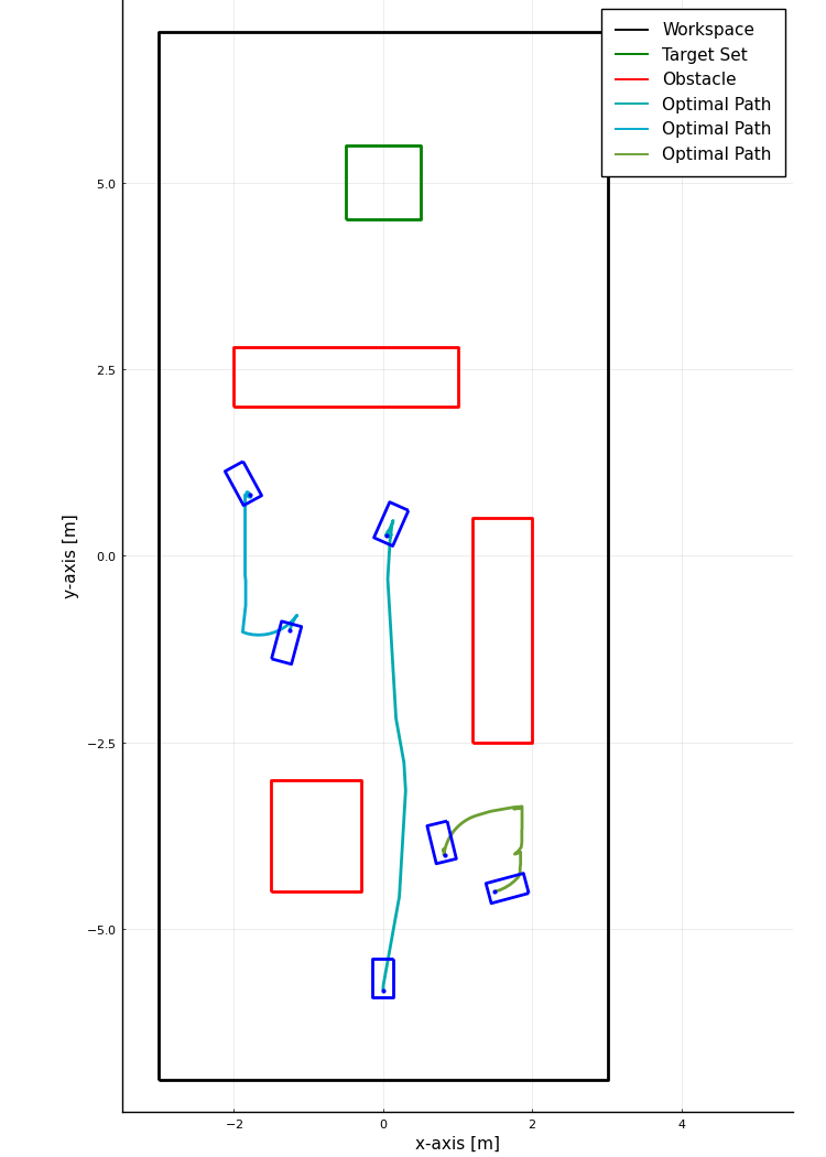
Solving HJB for Optimal Trajectories
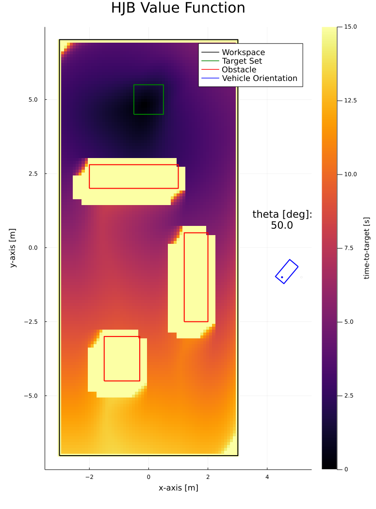
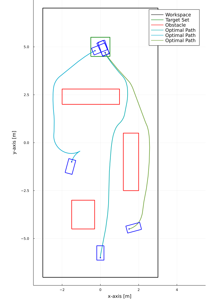
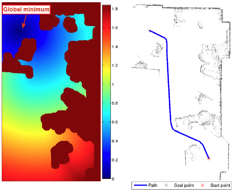
Value function from solving HJB PDE:
Optimal paths from gradient of value function:
Sliced at θ=50°
Solving HJB
- Apply system information to HJB PDE:
0 = \frac{\partial V}{\partial t} + \min_{u}\{\frac{\partial V}{\partial x}f(x,u) + C(x,u) \}
\frac{\partial V}{\partial t} = 0
C(x,u) = 1
- Value function doesn't change over time:
- Cost = time elapsed, cost rate:
-1 = \min_{u}\{\frac{\partial V}{\partial x} \cdot f(x,u) \}
-1 = \min_{(u_{v},u_{\phi})}\{V_{x}(u_{v}\cos{\theta}) + V_{y}(u_{v}\sin{\theta}) + V_{\theta}(u_{v}\frac{1}{l}\tan{u_{\phi}}) \}
Solving HJB
- Finite difference method (FDM) – numerical method for approximating derivatives
- Forward/backward:
V_{x} = \frac{V_{i+1,j,k} - V_{ijk}}{h_{xy}}
V_{x} = \frac{-(V_{i-1,j,k} - V_{ijk})}{h_{xy}}
\text{PDE: } -1 = \min_{(u_{v},u_{\phi})}\{V_{x}(u_{v}\cos{\theta}) + V_{y}(u_{v}\sin{\theta}) + V_{\theta}(u_{v}\frac{1}{l}\tan{u_{\phi}}) \}
- Upwind scheme
- Value at given state only depends on value of "upwind" states (closer to target)
- In FDM, need to pull value from upwind states
- Upwind direction is determined by state/action
i_{uw} = i + sgn(\dot{x}) \\
j_{uw} = j + sgn(\dot{y}) \\
k_{uw} = k + sgn(\dot{\theta})
V_{x} = \frac{sgn(\dot{x})(V_{i_{uw},j,k} - V_{ijk})}{h_{xy}}
Solving HJB
- Plugging in upwind FDM:
-1 = \frac{sgn(\dot{x})(V_{i_{uw}} - V)}{h_{xy}}(u_{v}\cos{\theta}) + \frac{sgn(\dot{y})(V_{j_{uw}} - V)}{h_{xy}}(u_{v}\sin{\theta}) + \frac{sgn(\dot{\theta})(V_{k_{uw}} - V)}{h_{\theta}}(u_{v}\frac{1}{l}\tan{u_{\phi}})
V_{i,j,k} = \frac{\frac{h_{xy}}{u_{v}} \text{ } + \text{ } V_{i_{uw},j,k} \text{ } s_{\dot{x}}\cos{\theta_{k}} \text{ } + \text{ } V_{i,j_{uw},k} \text{ } s_{\dot{y}}\sin{\theta_{k}} \text{ } + \text{ } V_{i,j,k_{uw}} \text{ } s_{\dot{\theta}}(\frac{h_{xy}}{h_{\theta}l})\tan{u_{\phi}}}{s_{\dot{x}}\cos{\theta_{k}} \text{ } + \text{ } s_{\dot{y}}\sin{\theta_{k}} \text{ } + \text{ } s_{\dot{\theta}}(\frac{h_{xy}}{h_{\theta}l})\tan{u_{\phi}}}
\text{PDE: } -1 = \min_{(u_{v},u_{\phi})}\{V_{x}(u_{v}\cos{\theta}) + V_{y}(u_{v}\sin{\theta}) + V_{\theta}(u_{v}\frac{1}{l}\tan{u_{\phi}}) \}
- Solution:
Solving HJB
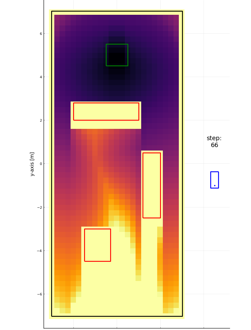
- Implementation:
- Set initial value at every node in grid (target: 0, else: large)
- Iterate through all nodes in free space
- Calculate V_ijk through FDM with upwind neighbors for each of 6 possible optimal actions, keep lowest value
- Repeat sweeps until all nodes have converged
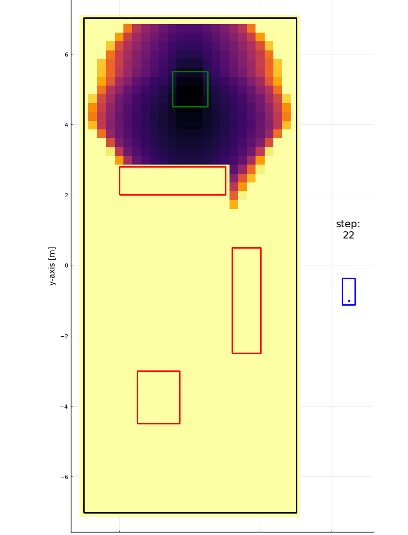
Step 22
Step 66
Results
h_{xy} = 0.25 \text{ m}
h_{xy} = 0.6 \text{ m}
h_{xy} = 0.1 \text{ m}
Results
h_{xy} = 0.25 \text{ m} \\
T_{path} = 7.66 \text{ s}
h_{xy} = 0.6 \text{ m} \\
T_{path} = \text{n/a}
h_{xy} = 0.1 \text{ m} \\
T_{path} = 7.45 \text{ s}
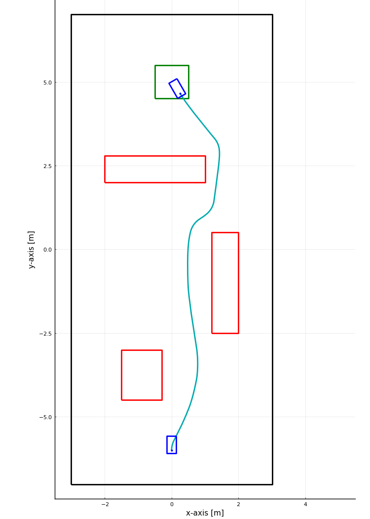
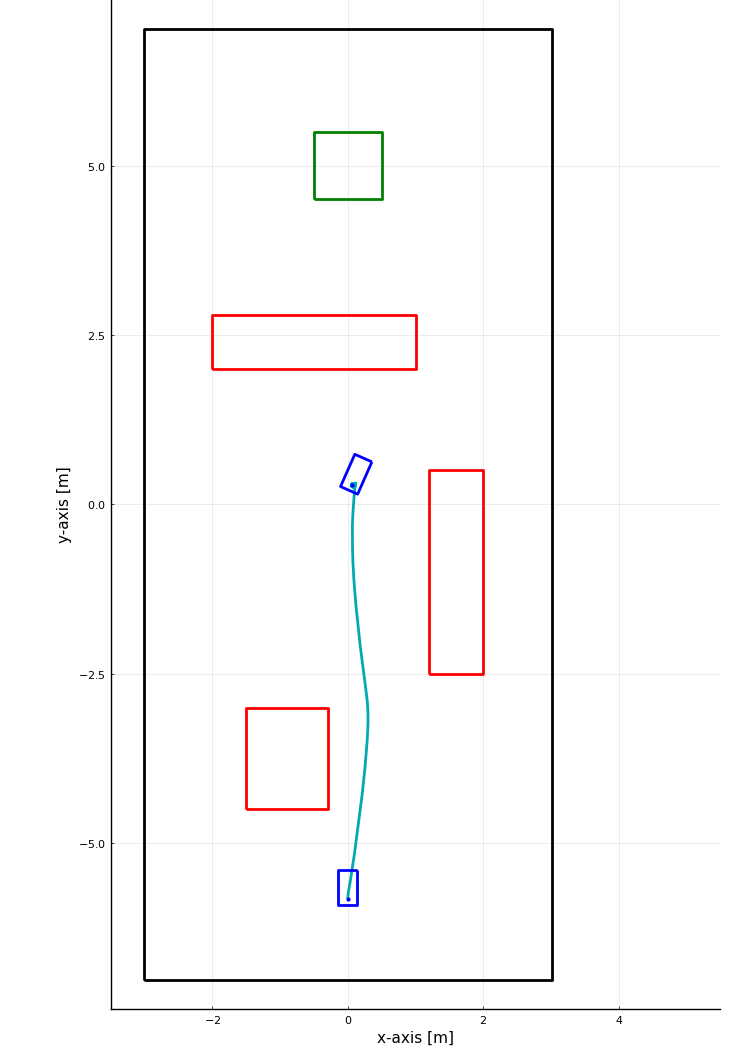
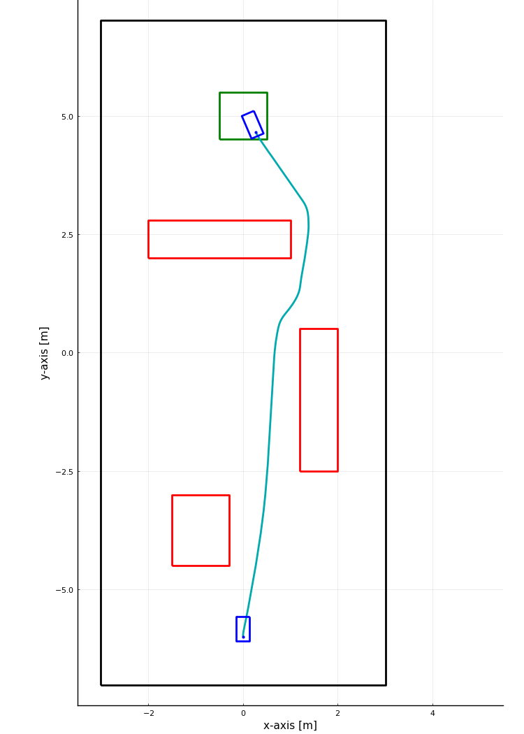
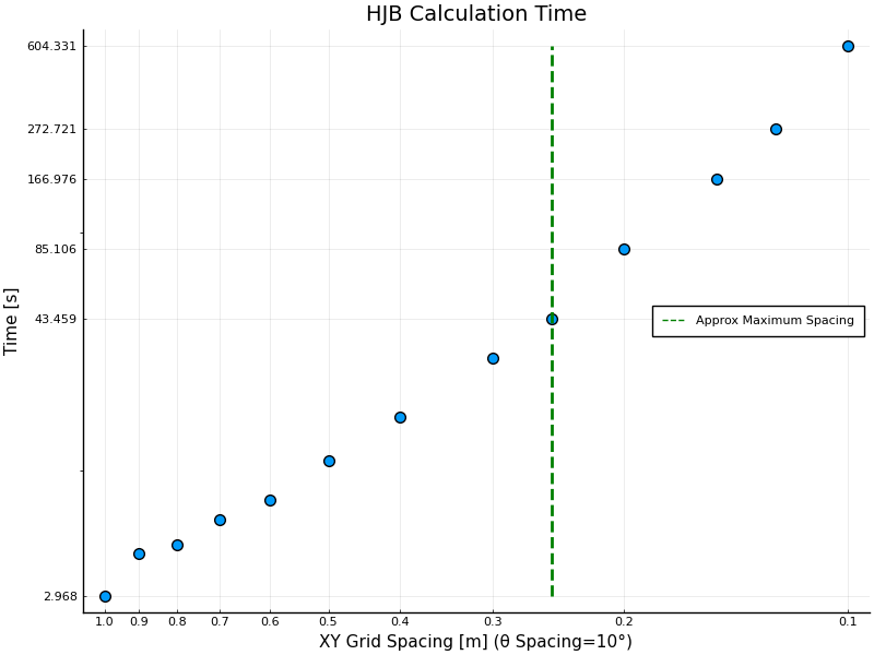
Results
- Runtime tracks number of nodes
- For given environment, need ~43 sec to calculate value at usable fidelity
- At lower resolution, gradient descent is unable to find usable paths
Issues
- Realistic scenarios may pose challenges in computation time:
- Larger environments
- Higher order dynamical models
- Lower power computing
- PDE solver is inflexible to changes in environment:
- Moving goal or adding obstacles requires completely recomputing HJB
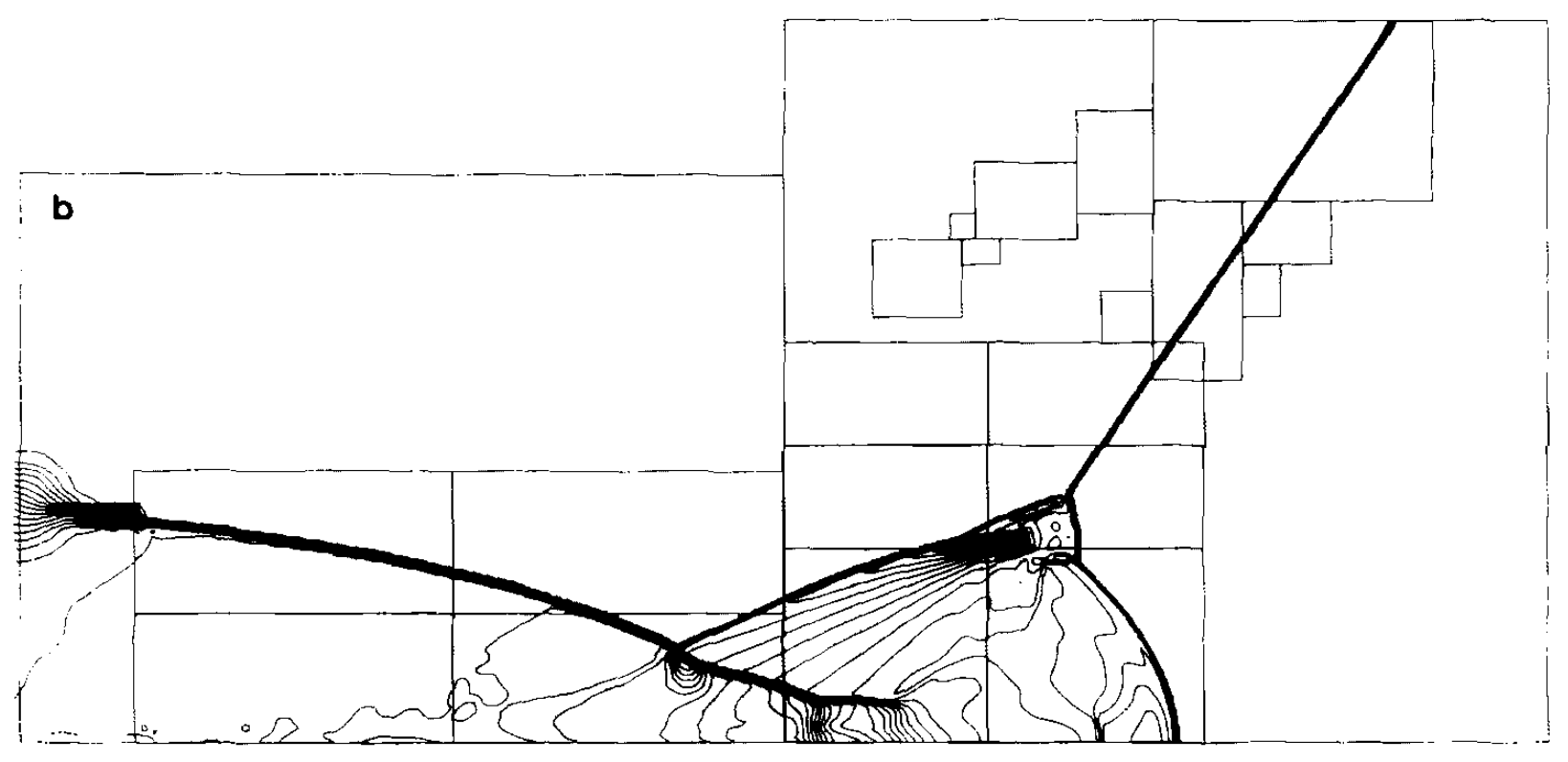
- Improvements:
- Adaptive mesh refinement
- Splitting methods
- Approximate value methods
Next Steps
- Past work:
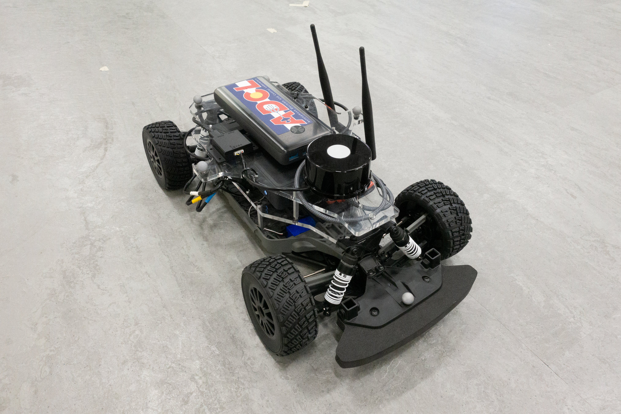
- HJB generator loaded on NUC
- HJB path planner implemented in ROS
- Current/future work:
- Refine existing HJB solver
- Investigate improvements
- Add velocity to state space
Copy of "Optimal Trajectories
By Zachary Sunberg


