
Breaking the Curse of Dimensionality in planning under uncertainty
Assistant Professor Zachary Sunberg
University of Colorado Boulder
Fall, 2024

Autonomous Decision and Control Laboratory

-
Algorithmic Contributions
- Scalable algorithms for partially observable Markov decision processes (POMDPs)
- Motion planning with safety guarantees
- Game theoretic algorithms
-
Theoretical Contributions
- Particle POMDP approximation bounds
-
Applications
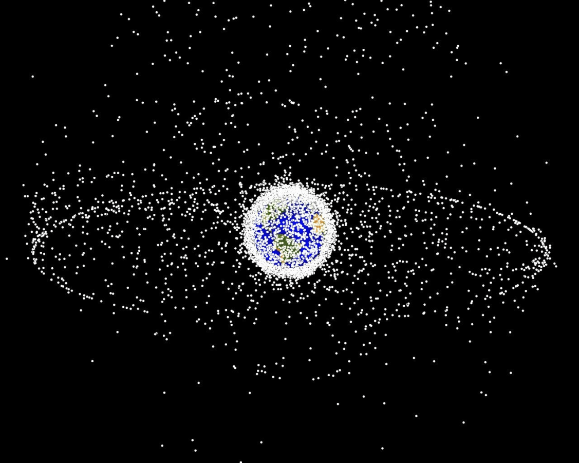
- Space Domain Awareness
- Autonomous Driving
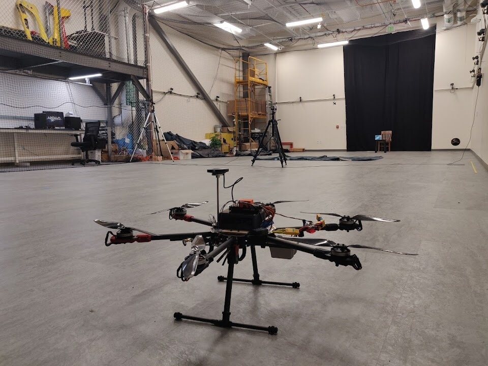
- Autonomous Aerial Scientific Missions
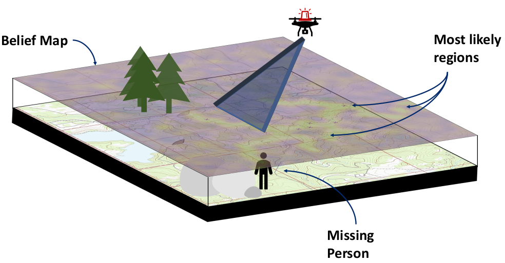
- Search and Rescue
- Space Exploration
- Ecology
-
Open Source Software
- POMDPs.jl Julia ecosystem

PI: Prof. Zachary Sunberg

PhD Students


Postdoc

Tweet by Nitin Gupta
29 April 2018
https://twitter.com/nitguptaa/status/990683818825736192
Example 1:
Autonomous Driving
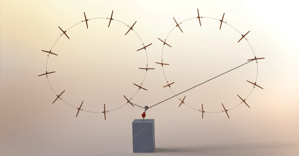
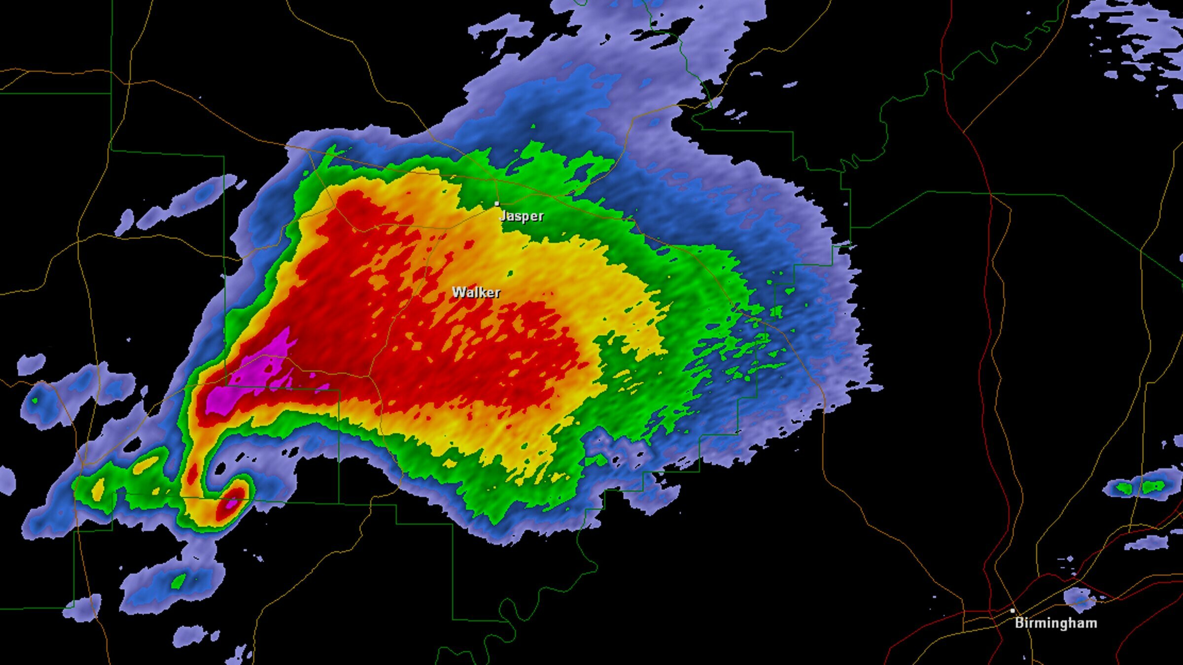
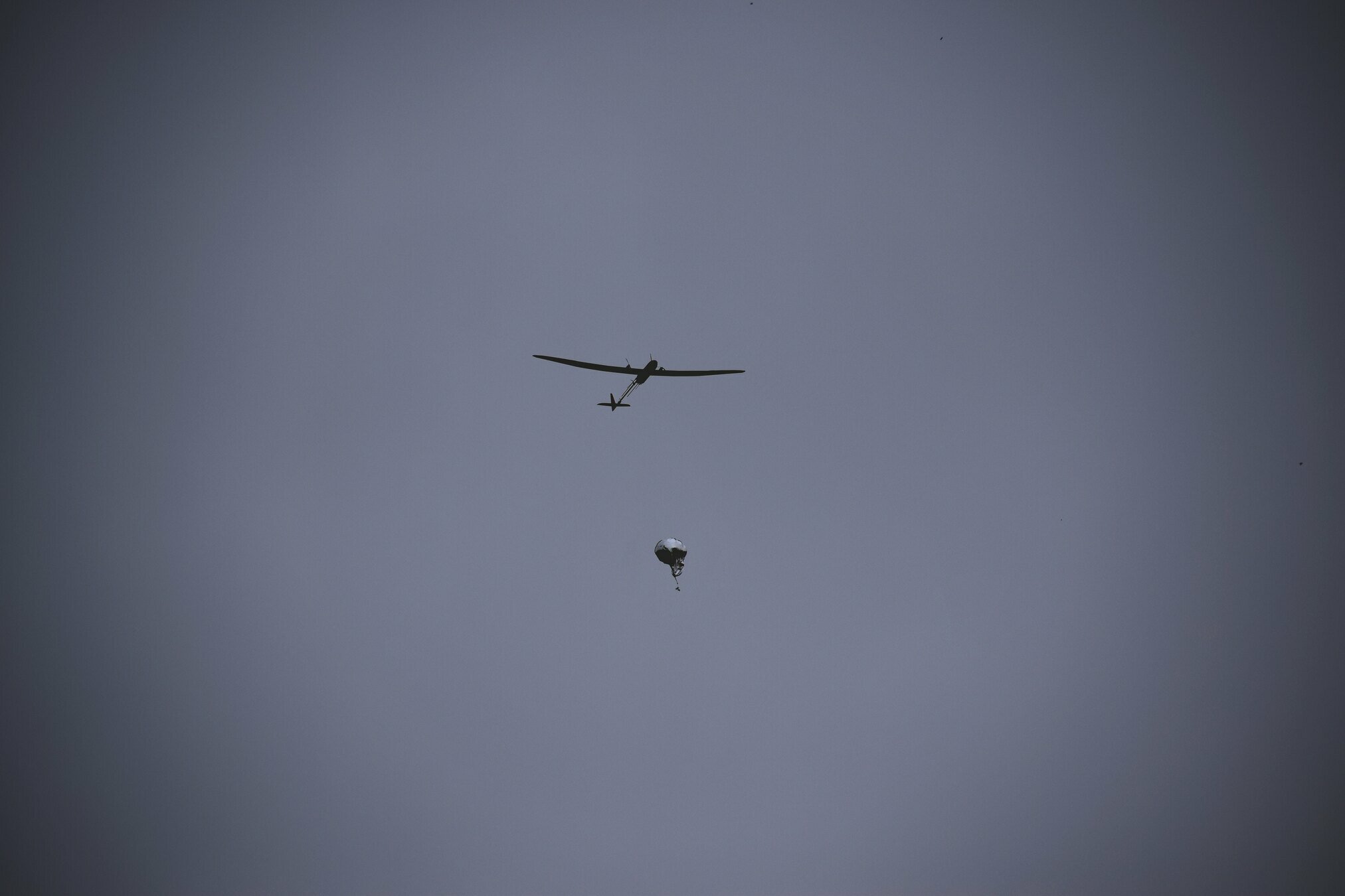
Example 2: Tornados
Video: Eric Frew
Example 2: Tornados
Video: Eric Frew
Example 2: Tornados
Video: Eric Frew
Example 2: Tornados

Example 3: Europa Lander

What do they have in common?
Driving: what are the other drivers going to do?
Tornado Forecasting: what is going on in the storm?
Europa: what is the system and environment status?
All are sequential decision-making problems with uncertainty!
All can be modeled as a POMDP.


Outline
- MDPs and POMDPs
- Solving POMDPs with tree search
- Breaking the curse of dimensionality
- Partially observable stochastic games
1. MDPs and POMDPs
Types of Uncertainty
Aleatory
Epistemic (Static)
Epistemic (Dynamic)


Interaction
MDP
RL
POMDP
Game
Markov Decision Process (MDP)
- \(\mathcal{S}\) - State space
- \(T(s' \mid s, a)\) - Transition probability distribution
- \(\mathcal{A}\) - Action space
- \(R(s, a)\) - Reward

Aleatory
\([x, y, z,\;\; \phi, \theta, \psi,\;\; u, v, w,\;\; p,q,r]\)
\(\mathcal{S} = \mathbb{R}^{12}\)
\[\underset{\pi:\, \mathcal{S} \to \mathcal{A}}{\text{maximize}} \quad \text{E}\left[ \sum_{t=0}^\infty R(s_t, a_t) \right]\]
Markov Decision Process (MDP)
Aleatory
\([x, y, z,\;\; \phi, \theta, \psi,\;\; u, v, w,\;\; p,q,r]\)
\(\mathcal{S} = \mathbb{R}^{12}\)
\(\mathcal{S} = \mathbb{R}^{12} \times \mathbb{R}^\infty\)
\[\underset{\pi:\, \mathcal{S} \to \mathcal{A}}{\text{maximize}} \quad \text{E}\left[ \sum_{t=0}^\infty R(s_t, a_t) \right]\]
- \(\mathcal{S}\) - State space
- \(T(s' \mid s, a)\) - Transition probability distribution
- \(\mathcal{A}\) - Action space
- \(R(s, a)\) - Reward
Reinforcement Learning
Aleatory
Epistemic (Static)
\([x, y, z,\;\; \phi, \theta, \psi,\;\; u, v, w,\;\; p,q,r]\)
\(\mathcal{S} = \mathbb{R}^{12}\)
\(\mathcal{S} = \mathbb{R}^{12} \times \mathbb{R}^\infty\)
- \(\mathcal{S}\) - State space
- \(T(s' \mid s, a)\) - Transition probability distribution
- \(\mathcal{A}\) - Action space
- \(R(s, a)\) - Reward
Partially Observable Markov Decision Process (POMDP)

- \(\mathcal{S}\) - State space
- \(T(s' \mid s, a)\) - Transition probability distribution
- \(\mathcal{A}\) - Action space
- \(R(s, a)\) - Reward
- \(\mathcal{O}\) - Observation space
- \(\mathcal{Z}(o \mid a, s')\): Observation probability distribution
Aleatory
Epistemic (Static)
Epistemic (Dynamic)
\([x, y, z,\;\; \phi, \theta, \psi,\;\; u, v, w,\;\; p,q,r]\)
\(\mathcal{S} = \mathbb{R}^{12}\)
\(\mathcal{S} = \mathbb{R}^{12} \times \mathbb{R}^\infty\)
\begin{aligned}
& \mathcal{S} = \mathbb{Z} \quad \quad \quad ~~ \mathcal{O} = \mathbb{R} \\
& s' = s+a \quad \quad o \sim \mathcal{N}(s, |s-10|) \\
& \mathcal{A} = \{-10, -1, 0, 1, 10\} \\
& R(s, a) = \begin{cases}
100 & \text{ if } a = 0, s = 0 \\
-100 & \text{ if } a = 0, s \neq 0 \\
-1 & \text{ otherwise}
\end{cases} & \\
\end{aligned}

State
Timestep
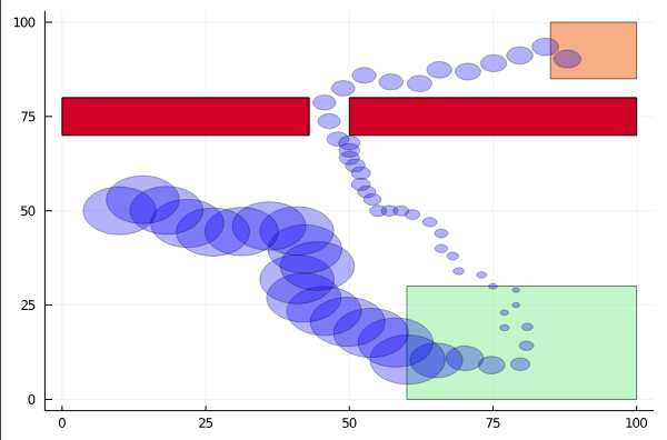
POMDP Example: Light-Dark
2. Solving POMDPs with Tree Search
Solving a POMDP
Environment
Belief Updater

True State
\(s = 7\)
Observation \(o = -0.21\)
\(b\)
\[b_t(s) = P\left(s_t = s \mid b_0, a_0, o_1 \ldots a_{t-1}, o_{t}\right)\]
\[ = P\left(s_t = s \mid b_{t-1}, a_{t-1}, o_{t}\right)\]
\(a\)
\[b_{t+1}(s') \propto Z(o \mid a, s')\int_{s \in \mathcal{S}} T(s' \mid s, a) b_t(s) ds\]
\(O(|\mathcal{S}|^2)\) for finite \(\mathcal{S}\)
\begin{aligned}
& \mathcal{S} = \mathbb{Z} \quad \quad \quad ~~ \mathcal{O} = \mathbb{R} \\
& s' = s+a \quad \quad o \sim \mathcal{N}(s, |s-10|) \\
& \mathcal{A} = \{-10, -1, 0, 1, 10\} \\
& R(s, a) = \begin{cases}
100 & \text{ if } a = 0, s = 0 \\
-100 & \text{ if } a = 0, s \neq 0 \\
-1 & \text{ otherwise}
\end{cases} & \\
\end{aligned}
State
Timestep
POMDP Example: Light-Dark
\begin{aligned}
& \mathcal{S} = \mathbb{Z} \quad \quad \quad ~~ \mathcal{O} = \mathbb{R} \\
& s' = s+a \quad \quad o \sim \mathcal{N}(s, |s-10|) \\
& \mathcal{A} = \{-10, -1, 0, 1, 10\} \\
& R(s, a) = \begin{cases}
100 & \text{ if } a = 0, s = 0 \\
-100 & \text{ if } a = 0, s \neq 0 \\
-1 & \text{ otherwise}
\end{cases} & \\
\end{aligned}
State
Timestep
Accurate Observations
Goal: \(a=0\) at \(s=0\)
Optimal Policy
Localize
\(a=0\)
POMDP Example: Light-Dark
Solving a POMDP
Environment
Belief Updater
Planner
\(a = +10\)
True State
\(s = 7\)
Observation \(o = -0.21\)

\(b\)
\[b_t(s) = P\left(s_t = s \mid b_0, a_0, o_1 \ldots a_{t-1}, o_{t}\right)\]
\[ = P\left(s_t = s \mid b_{t-1}, a_{t-1}, o_{t}\right)\]
\(Q(b, a)\)
Why are POMDPs difficult?
- Curse of History
- Curse of dimensionality
- State space
- Observation space
- Action space
Tree size: \(O\left(\left(|A||O|\right)^D\right)\)
Curse of Dimensionality
\(d\) dimensions, \(k\) segments \(\,\rightarrow \, |S| = k^d\)


1 dimension
e.g. \(s = x \in S = \{1,2,3,4,5\}\)
\(|S| = 5\)
2 dimensions
e.g. \(s = (x,y) \in S = \{1,2,3,4,5\}^2\)
\(|S| = 25\)
3 dimensions
e.g. \(s = (x,y,x_h) \in S = \{1,2,3,4,5\}^3\)
\(|S| = 125\)
(Discretize each dimension into 5 segments)

\(x\)
\(y\)
\(x_h\)

3. Breaking the Curse of Dimensionality
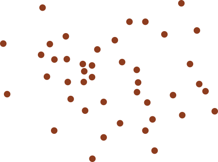
Integration
Find \(\underset{s\sim b}{E}[f(s)]\)
\[=\sum_{s \in S} f(s) b(s)\]
Monte Carlo Integration
\(Q_N \equiv \frac{1}{N} \sum_{i=1}^N f(s_i)\)
\(s_i \sim b\) i.i.d.
\(\text{Var}(Q_N) = \text{Var}\left(\frac{1}{N} \sum_{i=1}^N f(s_i)\right)\)
\(= \frac{1}{N^2} \sum_{i=1}^N\text{Var}\left(f(s_i)\right)\)
\(= \frac{1}{N} \text{Var}\left(f(s_i)\right)\)
\[P(|Q_N - E[f(s_i)]| \geq \epsilon) \leq \frac{\text{Var}(f(s_i))}{N \epsilon^2}\]
(Bienayme)
(Chebyshev)
Curse of dimensionality!
Particle Filter POMDP Approximation
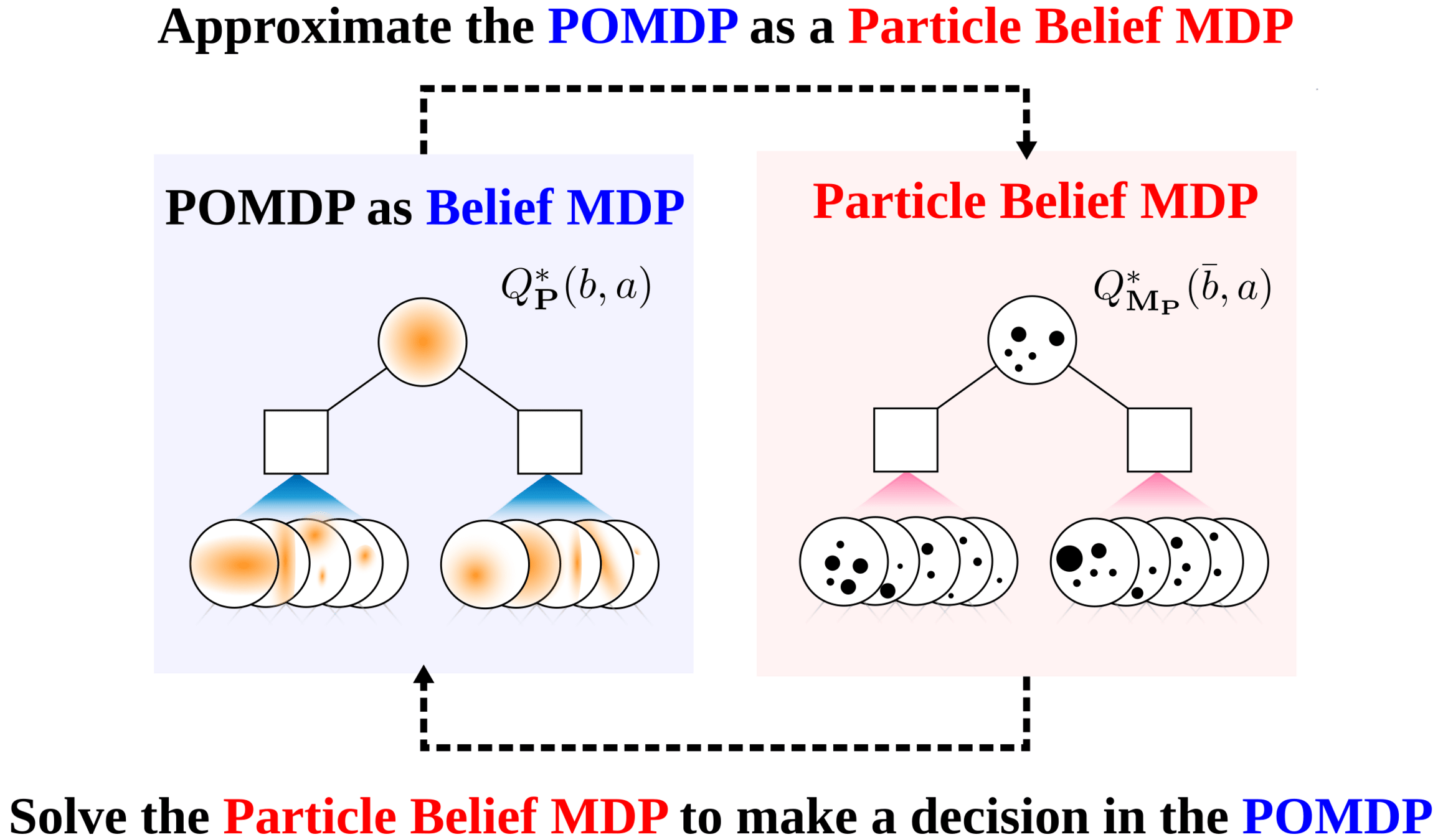
\[b(s) \approx \sum_{i=1}^N \delta_{s}(s_i)\; w_i\]
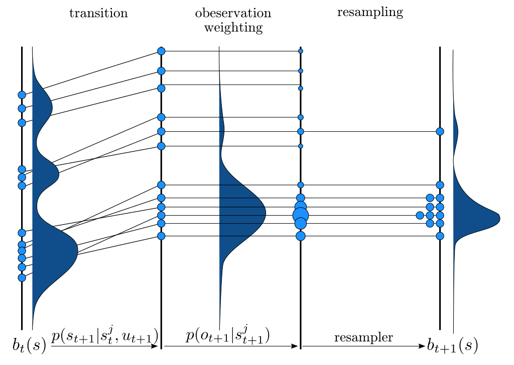
\[b_{t+1}(s') \propto Z(o \mid a, s')\int_{s \in \mathcal{S}} T(s' \mid s, a) b_t(s)\]
\(\implies\) Sample \(s'_i\) from \(T(s' | s_i, a)\),
\(w'_i \propto w_i \times Z(o \mid a, s'_i)\)

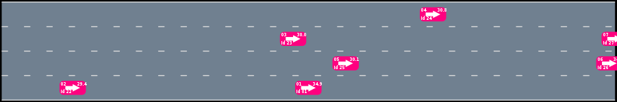
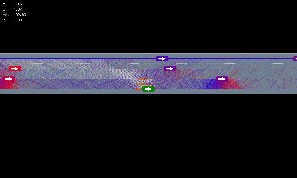
Example: Autonomous Driving
POMDP Formulation
\(s=\left(x, y, \dot{x}, \left\{(x_c,y_c,\dot{x}_c,l_c,\theta_c)\right\}_{c=1}^{n}\right)\)
\(o=\left\{(x_c,y_c,\dot{x}_c,l_c)\right\}_{c=1}^{n}\)
\(a = (\ddot{x}, \dot{y})\), \(\ddot{x} \in \{0, \pm 1 \text{ m/s}^2\}\), \(\dot{y} \in \{0, \pm 0.67 \text{ m/s}\}\)
R(s, a, s') = \text{in\_goal}(s') - \lambda \left(\text{any\_hard\_brakes}(s, s') + \text{any\_too\_slow}(s')\right)

Ego external state
External states of other cars
Internal states of other cars
External states of other cars
- Actions shielded (based only on external states) so they can never cause crashes
- Braking action always available
Efficiency
Safety


MDP trained on normal drivers


MDP trained on all drivers
Omniscient
POMCPOW (Ours)
Simulation results
[Sunberg & Kochenderfer, T-ITS 2023]
Convergence?
Key 1: Self Normalized Infinite Renyi Divergence Concentation
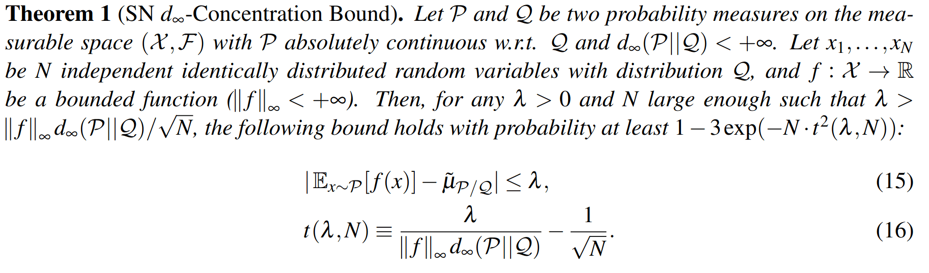
\(\mathcal{P}\): state distribution conditioned on observations (belief)
\(\mathcal{Q}\): marginal state distribution (proposal)
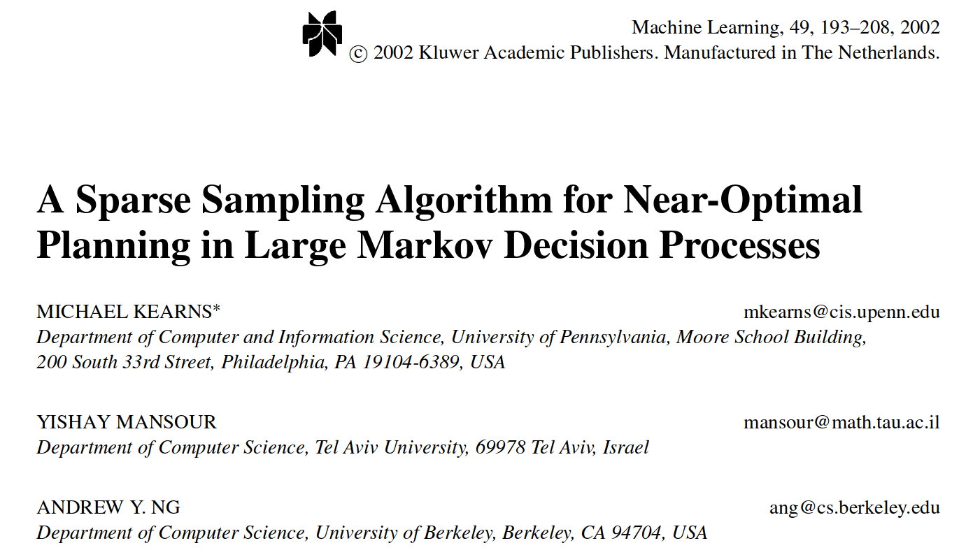
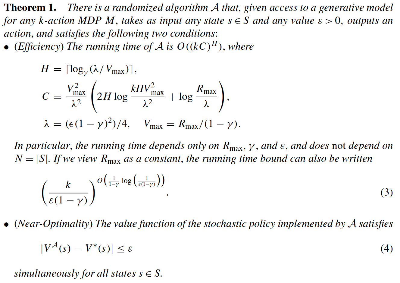
Key 2: Sparse Sampling
Expand for all actions (\(\left|\mathcal{A}\right| = 2\) in this case)
...
Expand for all \(\left|\mathcal{S}\right|\) states
\(C=3\) states
SS-\(\omega\) is close to Belief MDP
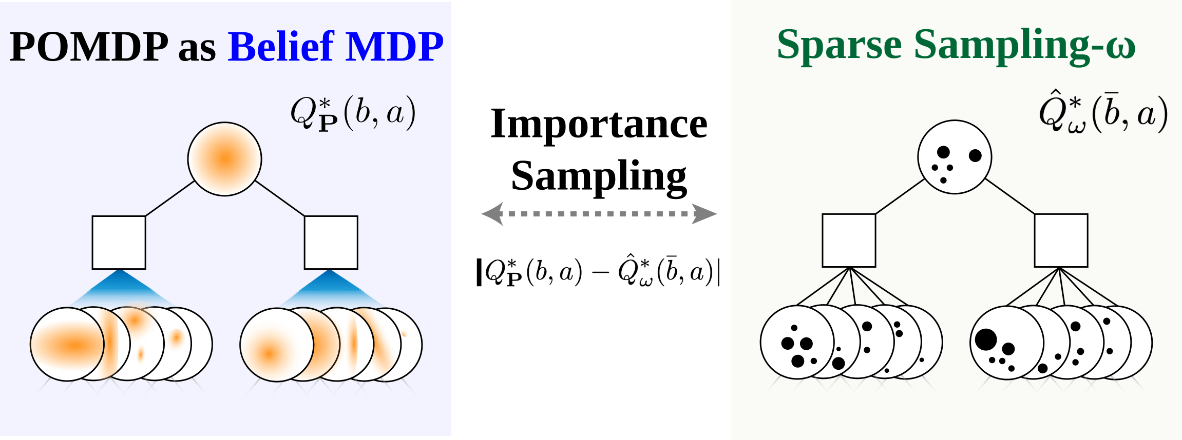
SS-\(\omega\) close to Particle Belief MDP (in terms of Q)

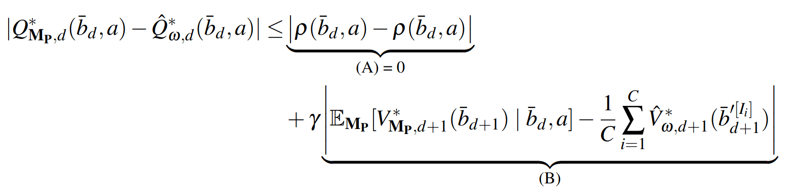
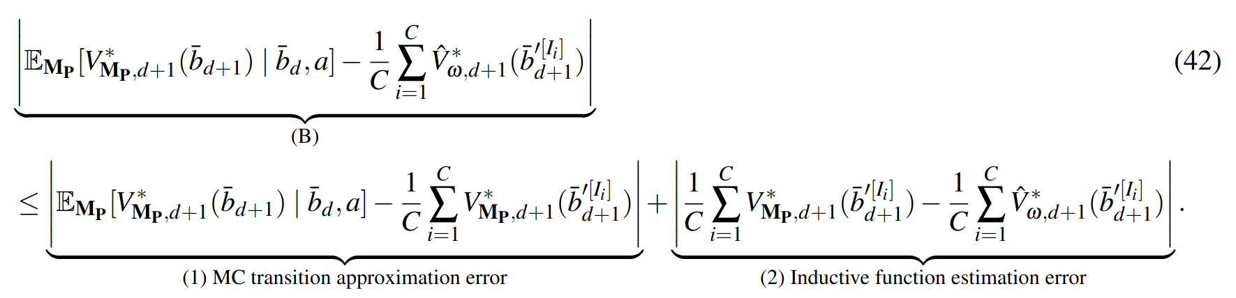
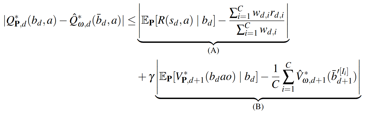
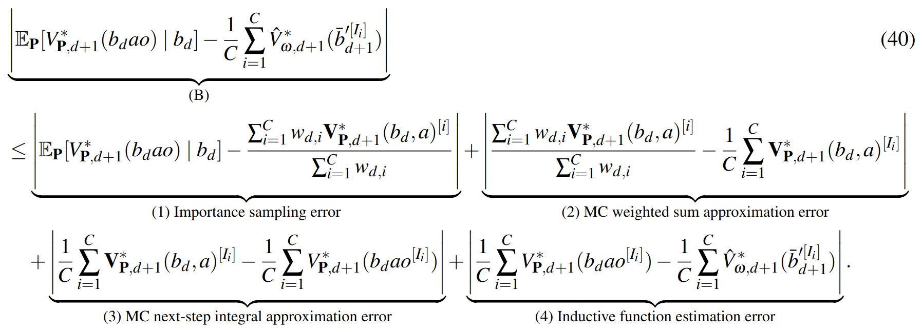
PF Approximation Accuracy
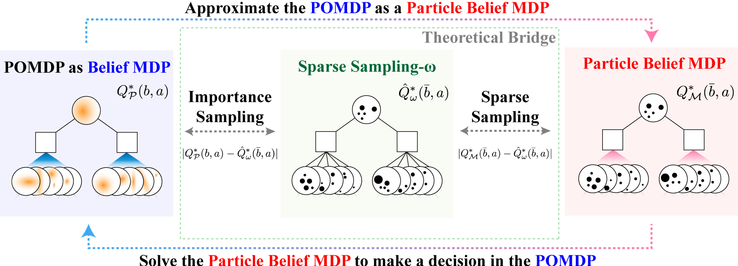
\[|Q_{\mathbf{P}}^*(b,a) - Q_{\mathbf{M}_{\mathbf{P}}}^*(\bar{b},a)| \leq \epsilon \quad \text{w.p. } 1-\delta\]
For any \(\epsilon>0\) and \(\delta>0\), if \(C\) (number of particles) is high enough,
[Lim, Becker, Kochenderfer, Tomlin, & Sunberg, JAIR 2023]
No direct dependence on \(|\mathcal{S}|\) or \(|\mathcal{O}|\)!

Particle belief planning suboptimality
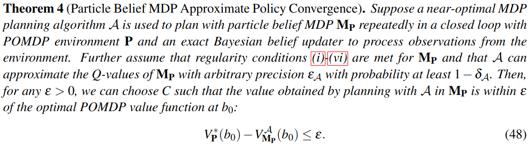
\(C\) is too large for any direct safety guarantees. But, in practice, works extremely well for improving efficiency.
[Lim, Becker, Kochenderfer, Tomlin, & Sunberg, JAIR 2023]
Why are POMDPs difficult?
- Curse of History
- Curse of dimensionality
- State space
- Observation space
- Action space

Tree size: \(O\left(\left(|A|C\right)^D\right)\)
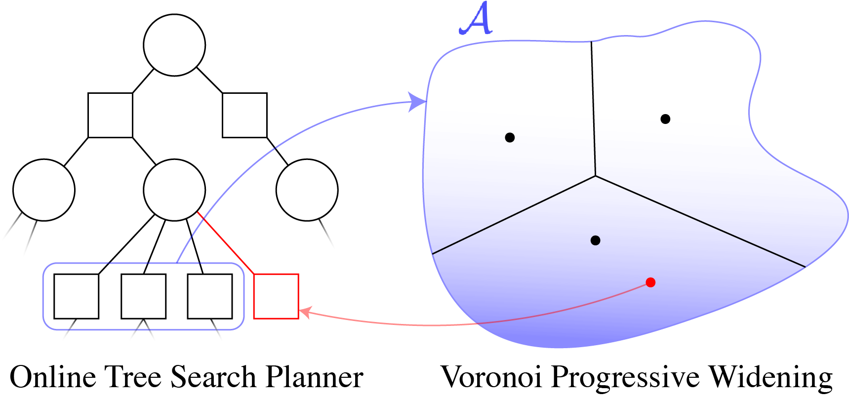
Solve simplified surrogate problem for policy deep in the tree
[Lim, Tomlin, and Sunberg, 2021]
Practical Safety Guarantees
Three Contributions
- Recursive constraints (solves "stochastic self-destruction")
- Undiscounted POMDP solutions for estimating probability
- Much faster motion planning with Gaussian uncertainty
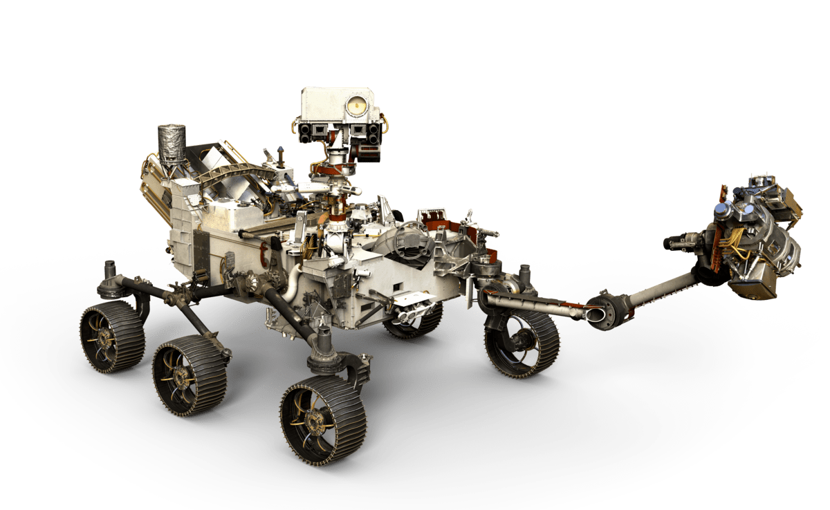

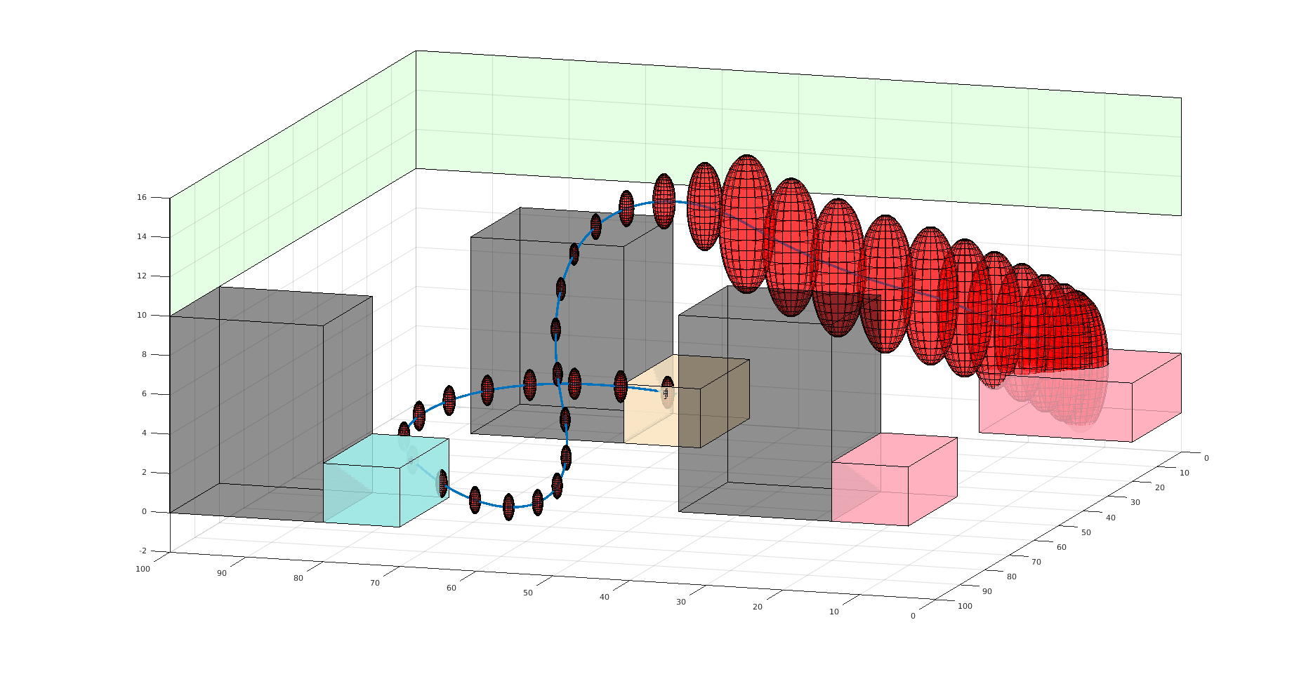
State:
- Position of rover
- Environment state: e.g. traversibility
- Internal status: e.g. battery, component health
[Ho et al., UAI 24], [Ho, Feather, Rossi, Sunberg, & Lahijanian, UAI 24], [Ho, Sunberg, & Lahijanian, ICRA 22]

4. Partially observable stochastic games (POSGs)
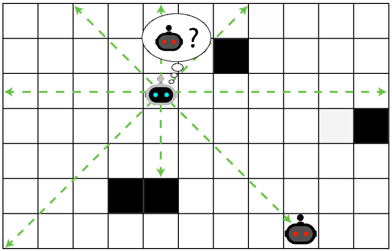
Laser Tag POMDP
Evader strategy:
Move away from pursuer
Embedded in \(T(s' \mid s, a)\)
Laser Tag POMDP
Partially Observable Markov Decision Process (POMDP)
- \(\mathcal{S}\) - State space
- \(T(s' \mid s, a)\) - Transition probability distribution
- \(\mathcal{A}\) - Action space
- \(R(s, a)\) - Reward
- \(\mathcal{O}\) - Observation space
- \(Z:\mathcal{S} \times \mathcal{A}\times \mathcal{S} \times \mathcal{O} \to \mathbb{R}\) - Observation probability distribution
Aleatory
Epistemic (Static)
Epistemic (Dynamic)
Partially Observable Stochastic Game (POSG)
Aleatory
Epistemic (Static)
Epistemic (Dynamic)
Interaction
- \(\mathcal{S}\) - State space
- \(T(s' \mid s, \bm{a})\) - Transition probability distribution
- \(\mathcal{A}^i, \, i \in 1..k\) - Action spaces
- \(R^i(s, \bm{a})\) - Reward function (cooperative, opposing, or somewhere in between)
- \(\mathcal{O}^i, \, i \in 1..k\) - Observation spaces
- \(Z(o^i \mid \bm{a}, s')\) - Observation probability distributions

Game Theory
Nash Equilibrium: All players play a best response.
Optimization Problem
\(\text{subject to} \quad g(x) \geq 0\)
\(\text{maximize} \quad f(x)\)
Game
Player 1: \(U_1 (a_1, a_2)\)
Player 2: \(U_2 (a_1, a_2)\)
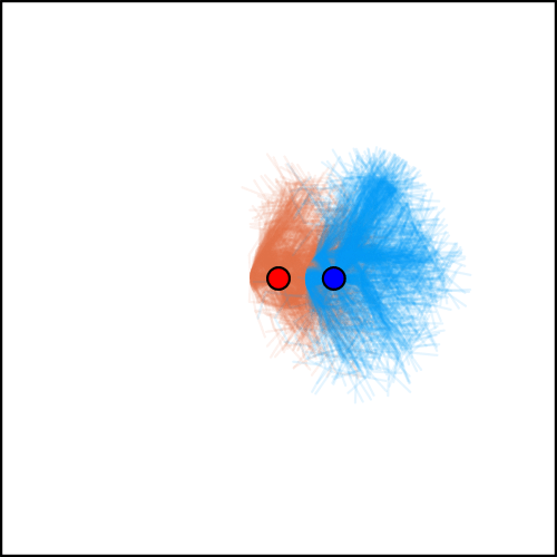
Collision
Example: Airborne Collision Avoidance
|
|
|
|
|
Player 1
Player 2
Up
Down
Up
Down
-6, -6
-1, 1
1, -1
-4, -4

Collision
Mixed Strategies
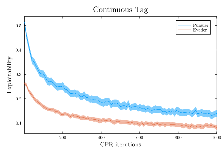
Nash Equilibrium \(\iff\) Zero Exploitability
\[\sum_i \max_{\pi_i'} U_i(\pi_i', \pi_{-i})\]
No Pure Nash Equilibrium!
Instead, there is a Mixed Nash where each player plays up or down with 50% probability.
If either player plays up or down more than 50% of the time, their strategy can be exploited.
Exploitability (zero sum):
Hypersonic Missile Defense (simplified)
|
|
|
|
|
Attacker
Defender
Up
Down
Up
Down
-1, 1
1, -1
1, -1
-1, 1
Collision
Collision
Strategy (\(\pi_i\)): probability distribution over actions
Belief-based approach


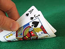
Finding a Nash Equilibrium: Poker
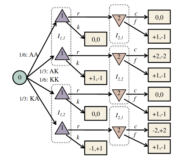
Image: Russel & Norvig, AI, a modern approach
P1: A
P1: K
P2: A
P2: A
P2: K
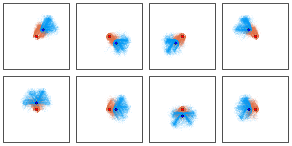
Conditional Distribution Info-set Tree (CDIT)
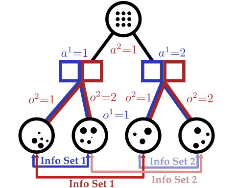
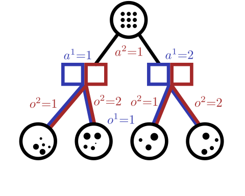
[Becker & Sunberg, In prep. for AAMAS '25]
Regret Matching
(External Sampling Counterfactual Regret Minimization)
\pi_{i}^{T+1}(\sigma')= \begin{cases}\frac{R_{i}^{T,+}(\sigma')}{\sum_{\sigma \in \Sigma_i} R_{i}^{T,+}(\sigma)} & \text { if } \sum_{\sigma \in \Sigma_i} R_{i}^{T,+}(\sigma)>0 \\ \frac{1}{|\Sigma_i|} & \text { otherwise. }\end{cases}
\bar{\pi}_i^T = \frac{1}{T}\sum_{t=1}^T\pi_i^t
Nash Equilibrium
Incentive to deviate makes a policy suboptimal
\delta(\pi) = \max_{\pi'}V(\pi') - V(\pi)
\delta(\pi) = 0 \implies V(\pi) = \max_{\pi'}V(\pi') = V^*
\delta^i(\pi^i, \pi^{-i}) = \max_{\pi^{i\prime}}V^i(\pi^{i\prime}, \pi^{-i}) - V^i(\pi^i, \pi^{-i})
\forall i,\delta^i(\pi) = 0 \implies \pi \text{ is a Nash equilibrium strategy}
For a single agent:
For multiple agents:
\text{NashConv}_A(\pi) = \sum_i \delta^i_A(\pi)
Regret Matching
\pi_{i}^{T+1}(\sigma')= \begin{cases}\frac{R_{i}^{T,+}(\sigma')}{\sum_{\sigma \in \Sigma_i} R_{i}^{T,+}(\sigma)} & \text { if } \sum_{\sigma \in \Sigma_i} R_{i}^{T,+}(\sigma)>0 \\ \frac{1}{|\Sigma_i|} & \text { otherwise. }\end{cases}
\bar{\pi}_i^T = \frac{1}{T}\sum_{t=1}^T\pi_i^t
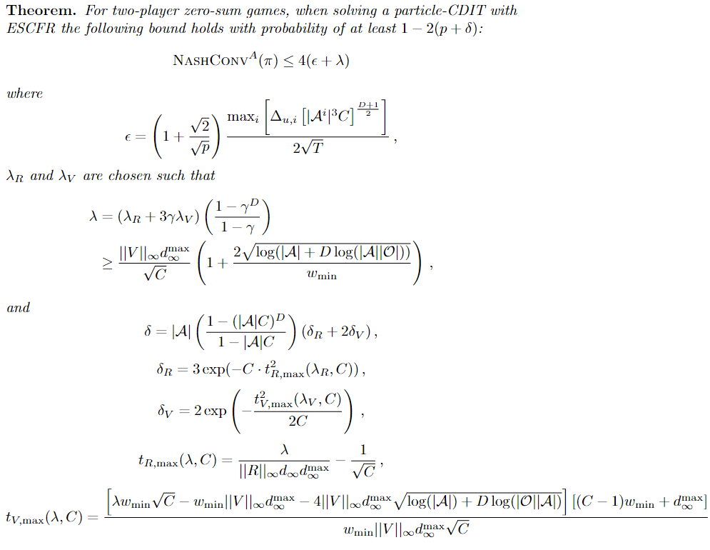
\max_i \delta^i(\bar{\pi}^T) \le \max_i \frac{R_i^T}{T}
Average regret bounds deviation incentive
[Becker & Sunberg, in prep for AAMAS '25]
Conditional Distribution Info-set Tree (CDIT)
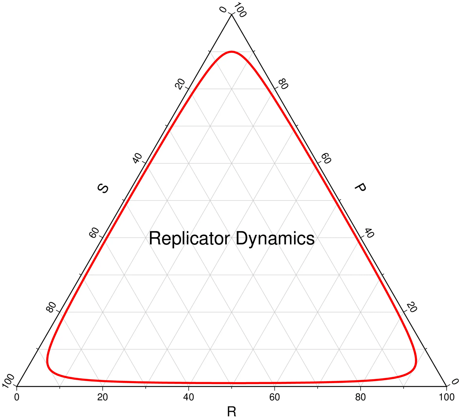
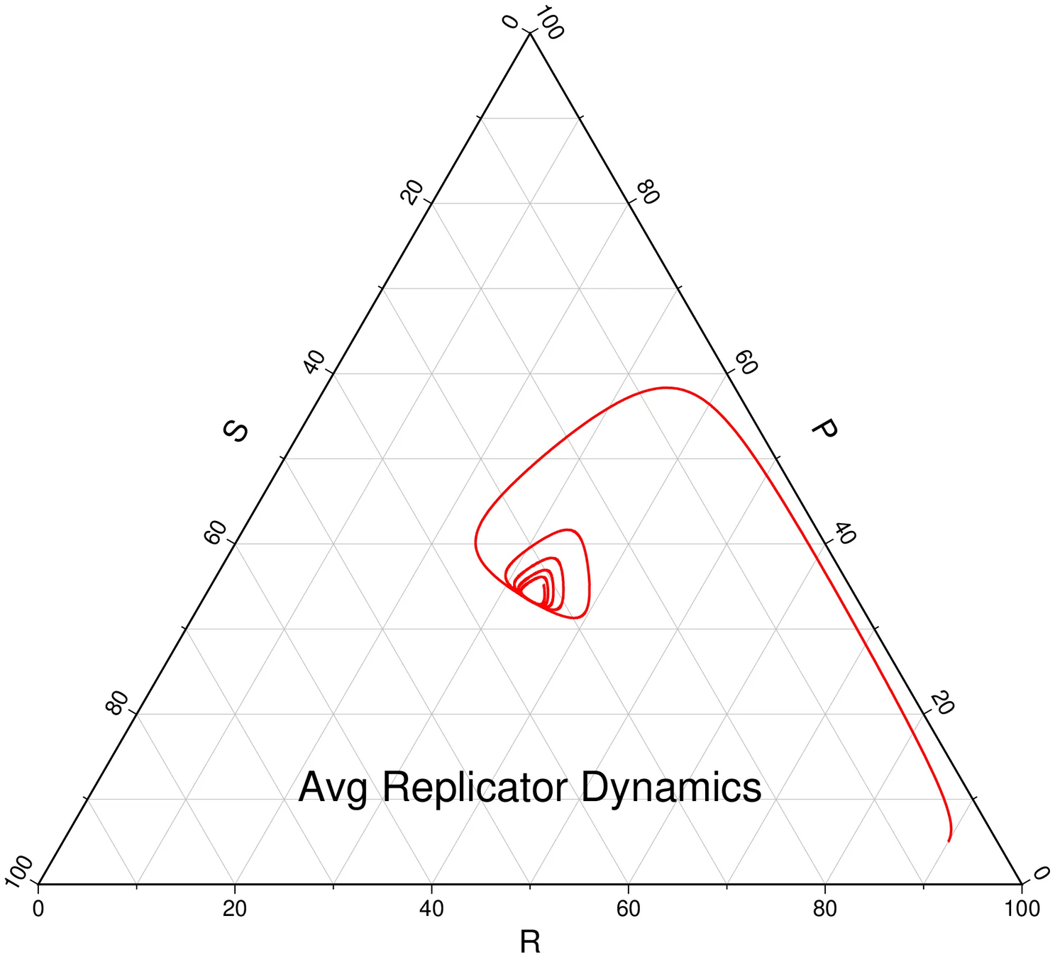
Convergence
| -1, -1 | -10, 0 | |
| 0, -10 | -5, -5 |
A
\(\sigma^1_1\)
\(\sigma^1_2\)
\(\ldots\)
\(\sigma^2_1\)
\(\sigma^2_2\)
\(\vdots\)
| -1.01, -1.20 | -9.82, 0.12 | |
| -0.10, -10.5 | -4.89, -5.02 |
\hat{A}
\(\sigma^1_1\)
\(\sigma^1_2\)
\(\ldots\)
\(\sigma^2_1\)
\(\sigma^2_2\)
\(\vdots\)
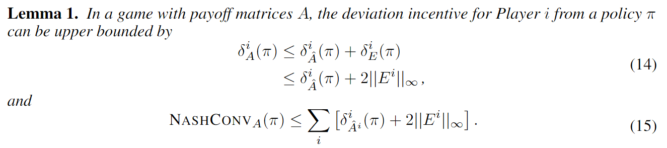
Incentive to deviate in approximate game \(\hat{A}\)
Maximum value approximation error (\(E^i = A^i - \hat{A}^i \))
Convergence Analysis for Games
V^1(\pi^1, \pi^2) = \mathbb{E}\left[\sum_{t=0}^\infty \gamma^t R^1(s_t, \pi^1(h_t^1), \pi^2(h_t^2))\right]
\delta^i(\pi^i, \pi^{-i}) = \max_{\pi^{i\prime}}V^i(\pi^{i\prime}, \pi^{-i}) - V^i(\pi^i, \pi^{-i})
\forall i,\delta^i(\pi) = 0 \implies \pi \text{ is a Nash eq.}
\text{NashConv}_A(\pi) = \sum_i \delta^i_A(\pi)
Incentive to deviate:
Takeaways
- POMDPs:
- If you have enough knowledge (e.g. sampleable T and explicit Z), solve as a particle belief MDP
- Don't worry too much about the curse of dimensionality in the state or observation space (Sparse sampling + particle filtering will help)
- Robust Guarantees are possible for small problems
- POSGs:
- Belief-based approaches are a losing battle
- One approach is CDIT - unifies particle-filtering POMDP methods
Thank You!


Funding orgs: (all opinions are my own)


VADeR
POMDP Planning with Learned Components
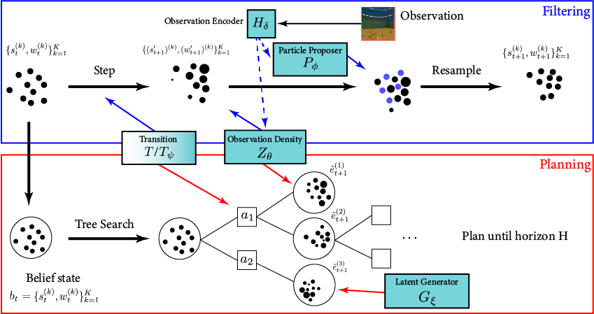
[Deglurkar, Lim, Sunberg, & Tomlin, 2023]
LANL Talk
By Zachary Sunberg


