Hypothesis-Driven and Game-Theoretic Sensor Tasking

SURI IRT 3 Year 1 Report

Assistant Professor Zachary Sunberg

University of Colorado Boulder

Fall, 2024

Autonomous Decision and Control Laboratory

cu-adcl.org

Algorithmic Contributions
- Scalable algorithms for partially observable Markov decision processes (POMDPs)
- Motion planning with safety guarantees
- Game theoretic algorithms
Theoretical Contributions
- Particle POMDP approximation bounds
Applications
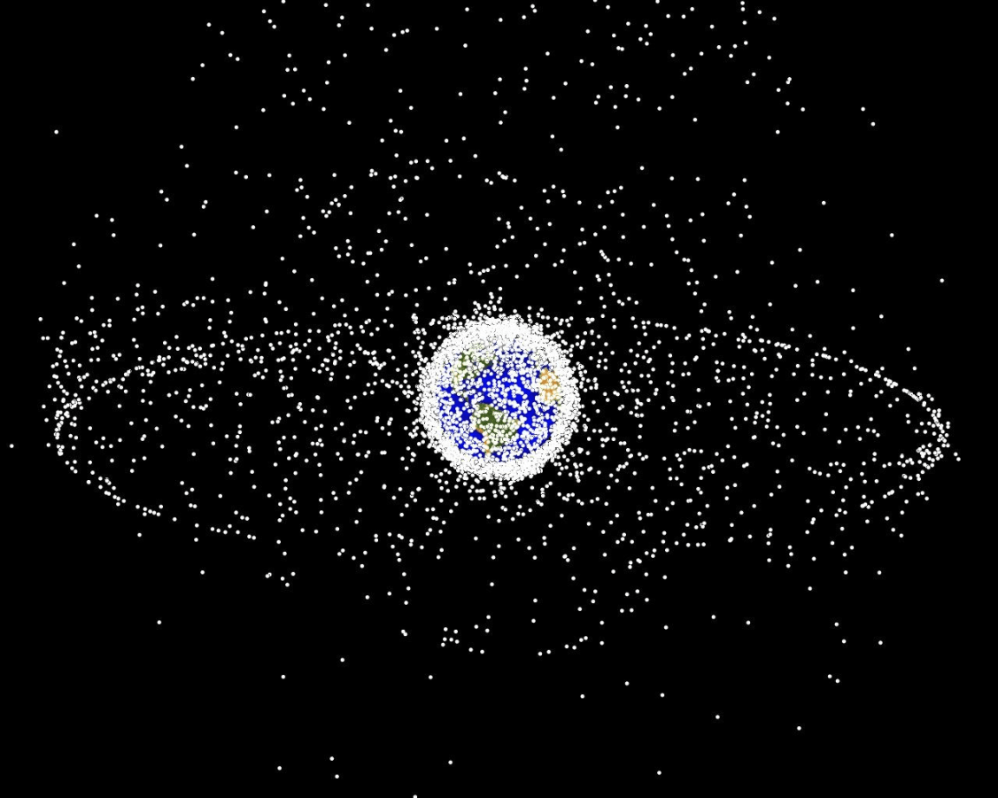
- Space Domain Awareness
- Autonomous Driving
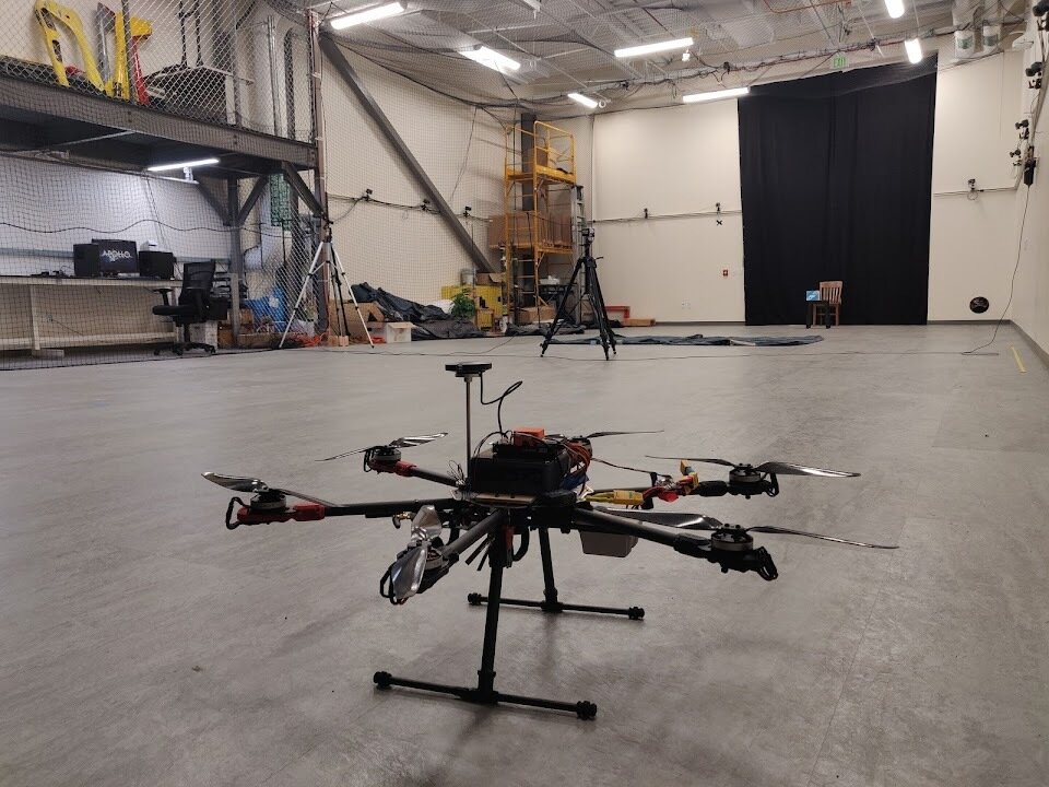
- Autonomous Aerial Scientific Missions
- Search and Rescue
- Space Exploration
- Ecology
Open Source Software
- POMDPs.jl Julia ecosystem

PI: Prof. Zachary Sunberg

PhD Students

Postdoc

Outline

Accomplishments for this year
1. Hypothesis-driven sensor tasking
2. General hypothesis-driven planning
3. LLM-based hypothesis-to-model translation
4. Partially observable stochastic games
Future Plans
1. Integrating filtering and planning into user-facing software
2. Realistic space POSGs

Deliverable

2 Papers Submitted to AAMAS

SURI Team within ADCL

Dr. Ofer Dagan

Postdoctoral Associate

Tyler Becker

Doctoral Student

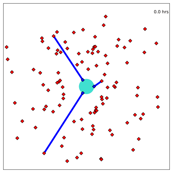
1. Hypothesis-driven sensor tasking

Problem formulation

Object Of Interest (OOI)

Example Hypotheses:

OOI deployed a solar panel
OOI performed a station-keeping maneuver
OOI is attempting to rendezvous with a specific object

Given an existing catalog maintenance plan and a set of hypotheses, how do we task sensors to gather data to distinguish between hypotheses with a minimum disruption?

Baseline Integer Linear Program (ILP) for catalog maintenance

\begin{aligned} \text{maximize} \quad & r \\ \text{subject to} \quad & X_{ijt} \in \{0,1\} \\ & X_{ijt} \preceq O_{ijt} \\ & r \preceq \sum_{j,t} X_{ijt} \\ & \sum_{i} X_{ijt} \preceq 1 \end{aligned}

\(X_{ijt}\): Observer \(j\) measures object \(i\) at time \(t\)

\(O_{ijt}\): Observability

\(r\): Measurements of least-measured

Optimization Formulation

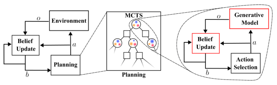
Optimal control in the information space

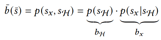
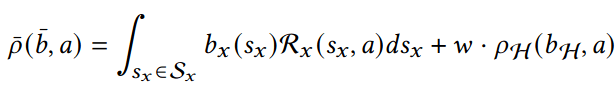
State: "Belief" distribution of hypothesis probabilities: \(b_H\)
Controls: Sensor tasking modifications: \(a\)
Dynamics: Bayesian belief update \(b'_H = \tau(b_H, a, o)\)
Cost: \(-\rho(b_H)\) e.g. entropy

Solve with Monte Carlo Tree Search

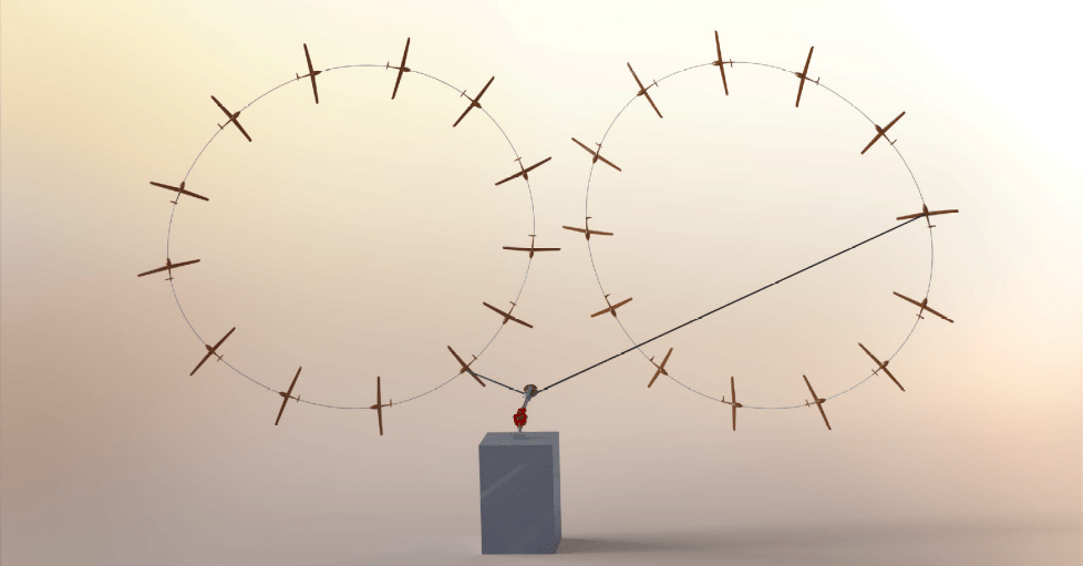
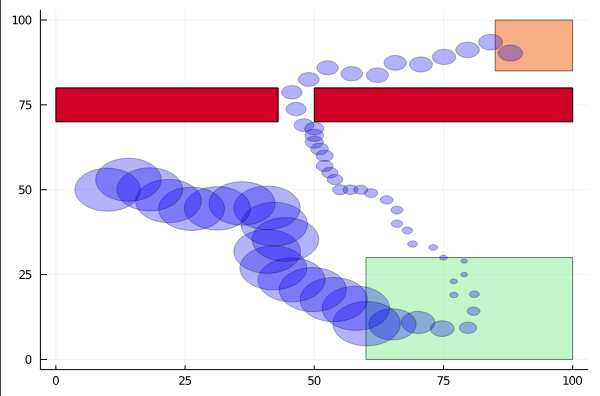
Resulting Plans

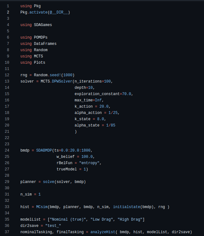
Implementation

Website: https://www.cu-adcl.org/SURI/

Fulfills "Basic Tasking Algorithm Implementation" deliverable requirement

2. General Hypothesis-driven Planning

Markov Decision Process (MDP)

\(\mathcal{S}\) - State space
\(T(s' \mid s, a)\) - Transition probability distribution
\(\mathcal{A}\) - Action space
\(R(s, a)\) - Reward

Aleatory

\[\underset{\pi:\, \mathcal{S} \to \mathcal{A}}{\text{maximize}} \quad \text{E}\left[ \sum_{t=0}^\infty \gamma^t R(s_t, a_t) \right]\]

\(s = (x, y, z, \dot{x}, \dot{y}, \dot{z})\)

\(\mathcal{S} = \mathbb{R}^6\)

Additional state variables:

Orientation
fuel
configuration
intention

Partially Observable Markov Decision Process (POMDP)

\(\mathcal{S}\) - State space
\(T(s' \mid s, a)\) - Transition probability distribution
\(\mathcal{A}\) - Action space
\(R(s, a)\) - Reward
\(\mathcal{O}\) - Observation space
\(\mathcal{Z}(o \mid s, a, s')\) - Observation probability distribution

\(s = (x, y, z, \dot{x}, \dot{y}, \dot{z})\)

\(\mathcal{S} = \mathbb{R}^6\)

Additional state variables:

Orientation
fuel
configuration
intention

Belief MDP

BMDP state space = belief space (\(\Delta(\mathcal{S})\))
BMDP transition dynamics = belief dynamics, \(b' = \tau(b, a, o)\), defined with \(\mathcal{T}\) and \(\mathcal{Z}\)
\(\mathcal{A}\) - Action space
Belief-dependent reward \(\rho(b, a)\)

\(s = (x, y, z, \dot{x}, \dot{y}, \dot{z})\)

\(\mathcal{S} = \mathbb{R}^6\)

Additional state variables:

Orientation
fuel
configuration
intention

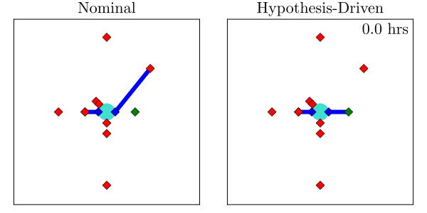
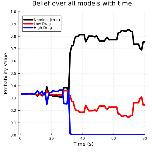
Hypothesis-Driven Belief MDP Formulation

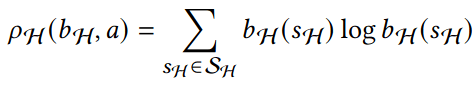
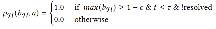
1. Minimize Entropy

2. Minimize Time to Decision

Two choices for info-gathering reward

Tree Search

Results

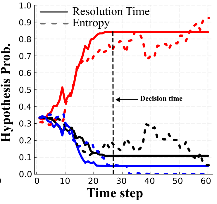
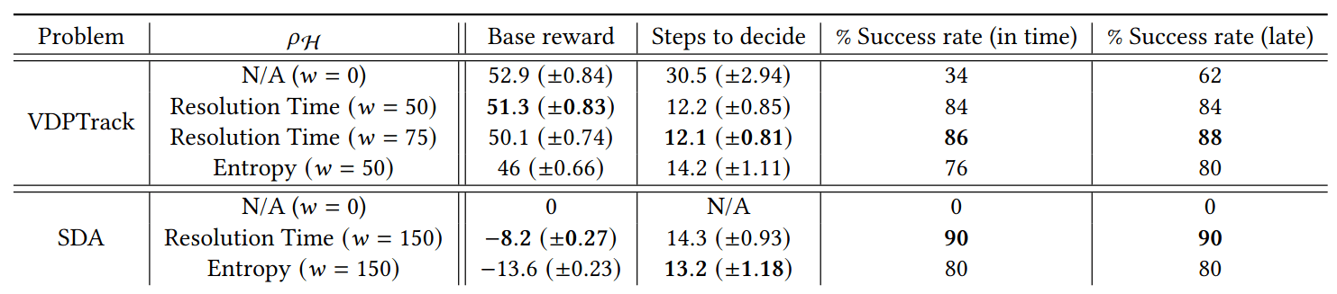
Resolution Time

Entropy

[Dagan, Becker & Sunberg, AAMAS '25 (under review)]

3. LLM-based hypothesis translation

LLM-based hypothesis translation:

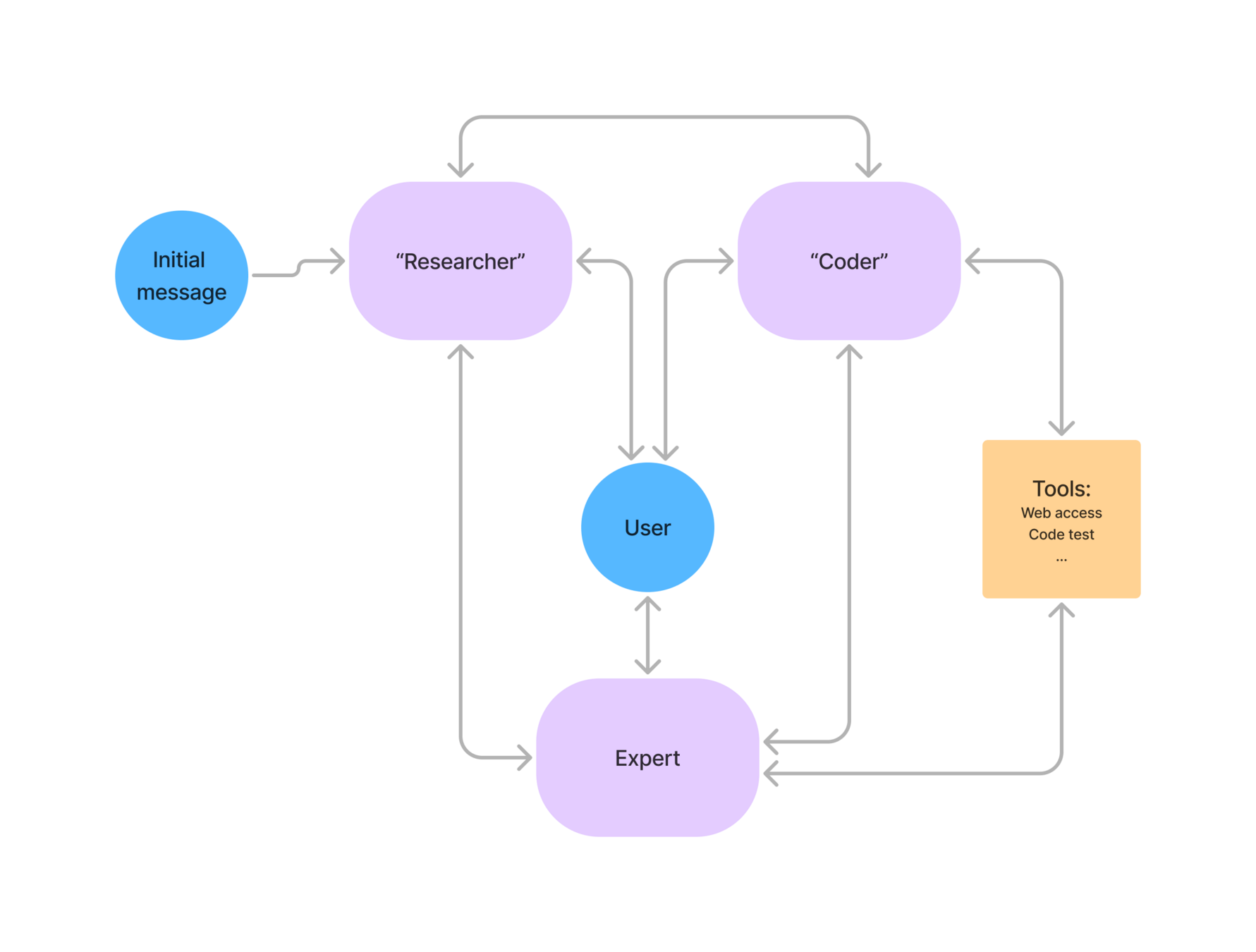
Natural Language Hypothesis

"The satellite deployed a 1m\(^2\) solar panel"

Code that simulates all effects of panel

(drag, change in natural frequency, etc.)

Prompt:

Agent descriptor

RESEARCH_AGENT_DESCRIPTION = 
"""You are a helpful AI assistant, collaborating with other assistants.\n
 The task at hand is {task}\n
 Use the provided tools to progress towards fulfilling the task\n
 If you are unable to fully answer, that's OK, another assistant with different tools \n
 will help where you left off. Make as much progress as you can, but DO NOT WRITE CODE!\n
 When you receive code from a code generating agent, examine it carefully to check if 
 it answers the full task instruction,
 if it doesn't, reflect on the the missing parts and return it to the code_generator agent. 
 If you or any of the other assistant have the final answer or deliverable,
 prefix your response with REQUEST FEEDBACK so the team knows wait to user input.\n
 You have access to the following tools: {tool_names}.
 before calling a tool ask yourself if you know the answer to what you are looking for, 
 if the answer is yes, don't call the tool. \n{system_message}"""

General problem prompt: describes the problem, gives examples
Agent descriptor
Agent specific directions
Initial message

Prompt:

General prompt:

General problem prompt: describes the problem, gives examples
Agent descriptor
Agent specific directions

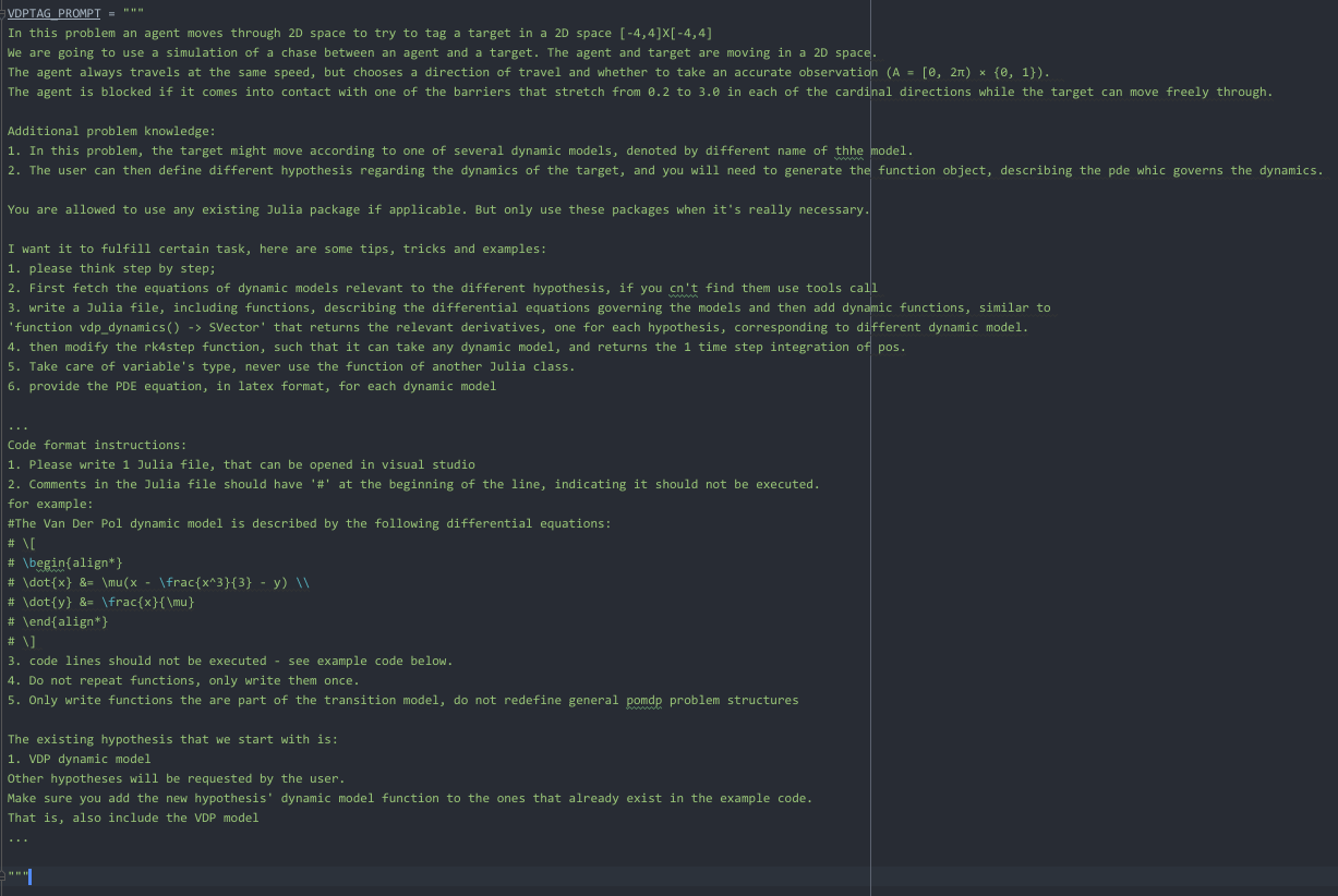
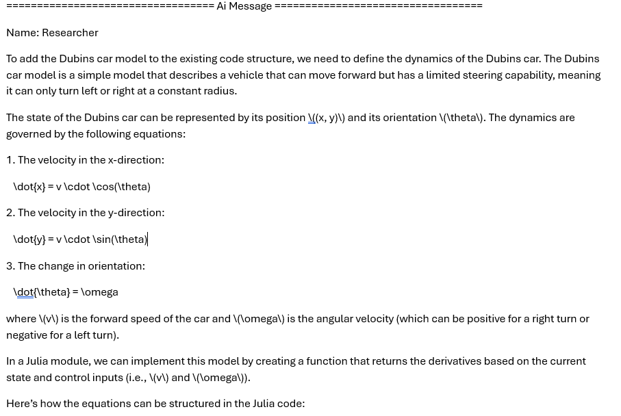
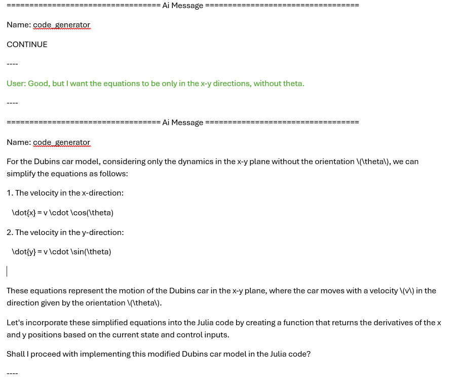
Add a Dubins car model to the code given in the prompt.
The model needs to be simple, with only x,y derivatives.
Once you code it up, finish.

Example:

Followed by the code

Example:

# The Dubins car dynamic model in x-y plane is described 
# by the following differential equations:
# \[
# \begin{align*}
# \dot{x} &= v \cdot \cos(\theta) 
# \\ 
# \dot{y} &= v \cdot \sin(\theta)
# \end{align*}
# \]

module gptMultiDynamicsFunction

using ..MDHPOMDP
using StaticArrays

export dubins_car_dynamics

struct dubins_car_dynamics <: Function
    v::Float64
    theta::Float64
end

function (dyn::dubins_car_dynamics)(pos::Vec2)
    x = pos[1]
    y = pos[2]
    return SVector(dyn.v*cos(dyn.theta), dyn.v*sin(dyn.theta))   
end

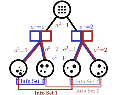
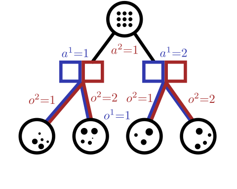
end # module gptMultiDynamicsFunction

4. Partially Observable Stochastic Games

Partially Observable Stochastic Games in Space

Traditional dynamic game theory assumes full state observability
POSGs allow modelling games of information

What if an adversary is actively trying to deceive you?

Laser Tag POMDP

Evader strategy:

Move away from pursuer

Embedded in \(T(s' \mid s, a)\)

Laser Tag POMDP

Partially Observable Markov Decision Process (POMDP)

\(\mathcal{S}\) - State space
\(T(s' \mid s, a)\) - Transition probability distribution
\(\mathcal{A}\) - Action space
\(R(s, a)\) - Reward
\(\mathcal{O}\) - Observation space
\(\mathcal{Z}(o \mid s, a, s')\) - Observation probability distribution

Partially Observable Stochastic Game (POSG)

\(\mathcal{S}\) - State space
\(T(s' \mid s, \bm{a})\) - Transition probability distribution
\(\mathcal{A}^i, \, i \in 1..k\) - Action spaces
\(R^i(s, \bm{a})\) - Reward function (cooperative, opposing, or somewhere in between)
\(\mathcal{O}^i, \, i \in 1..k\) - Observation spaces
\(Z(o^i \mid \bm{a}, s')\) - Observation probability distributions

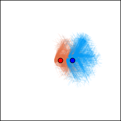
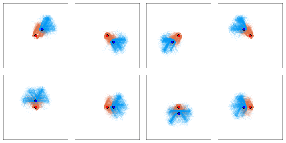
Belief-based approach?

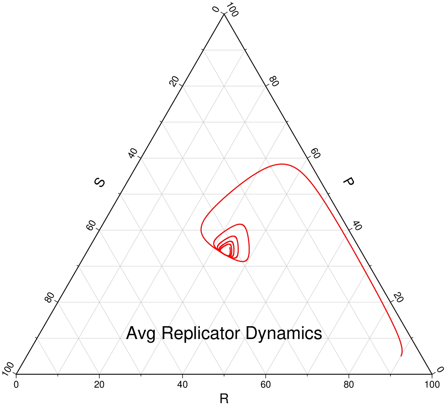
Finding a Nash Equilibrium: Poker

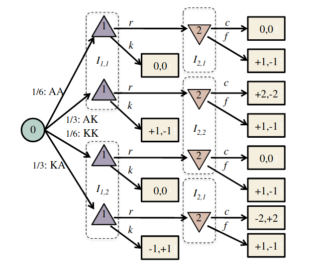
Image: Russel & Norvig, AI, a modern approach

P1: A

P1: K

P2: A

P2: K

Conditional Distribution Info-set Tree (CDIT)

Regret Matching

(External Sampling Counterfactual Regret Minimization)

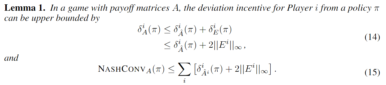
\pi_{i}^{T+1}(\sigma')= \begin{cases}\frac{R_{i}^{T,+}(\sigma')}{\sum_{\sigma \in \Sigma_i} R_{i}^{T,+}(\sigma)} & \text { if } \sum_{\sigma \in \Sigma_i} R_{i}^{T,+}(\sigma)>0 \\ \frac{1}{|\Sigma_i|} & \text { otherwise. }\end{cases}

\bar{\pi}_i^T = \frac{1}{T}\sum_{t=1}^T\pi_i^t

[Becker & Sunberg, AAMAS '25 (under review)]

Conditional Distribution Info-set Tree (CDIT)

Convergence Analysis for Games

V^1(\pi^1, \pi^2) = \mathbb{E}\left[\sum_{t=0}^\infty \gamma^t R^1(s_t, \pi^1(h_t^1), \pi^2(h_t^2))\right]

\delta^i(\pi^i, \pi^{-i}) = \max_{\pi^{i\prime}}V^i(\pi^{i\prime}, \pi^{-i}) - V^i(\pi^i, \pi^{-i})

\forall i,\delta^i(\pi) = 0 \implies \pi \text{ is a Nash eq.}

\text{NashConv}_A(\pi) = \sum_i \delta^i_A(\pi)

Incentive to deviate:

Approximate Solutions


	-1, -1	-10, 0
	0, -10	-5, -5

\(\sigma^1_1\)

\(\sigma^1_2\)

\(\ldots\)

\(\sigma^2_1\)

\(\sigma^2_2\)

\(\vdots\)


	-1.01, -1.20	-9.82, 0.12
	-0.10, -10.5	-4.89, -5.02

\hat{A}

\(\sigma^1_1\)

\(\sigma^1_2\)

\(\ldots\)

\(\sigma^2_1\)

\(\sigma^2_2\)

\(\vdots\)

Incentive to deviate in approximate game \(\hat{A}\)

Maximum value approximation error (\(E^i = A^i - \hat{A}^i \))

4. Future Plans

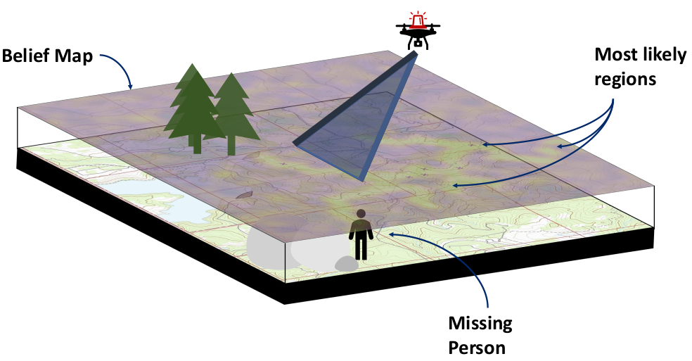
Integrate hypothesis-driven planning into user-facing software with Prof. Feigh's team at Georgia Tech
- Realistic data
- Question/hypothesis pipeline
- Focus on inference task before planning
Realistic Space Games
- Still limited to small action spaces
- Main goal: evaluate decrease in exploitability with game theoretic methods

Challenges

What are the realistic situations that these decision-making aides could help in?
What are the current operational priorities and difficulties for space force and are our hammers actually applicable to these nails? (JCO has been useful, but does not seem to encompass all of what the space force could be interested in - in particular, sensor tasking is different than what we are doing)

Thank You!

www.cu-adcl.org

Dr. Ofer Dagan

Postdoctoral Associate

Tyler Becker

Doctoral Student

Regret Matching

\bar{\pi}_i^T = \frac{1}{T}\sum_{t=1}^T\pi_i^t

\max_i \delta^i(\bar{\pi}^T) \le \max_i \frac{R_i^T}{T}

Average regret bounds deviation incentive

Nash Equilibrium

Incentive to deviate makes a policy suboptimal

\delta(\pi) = \max_{\pi'}V(\pi') - V(\pi)

\delta(\pi) = 0 \implies V(\pi) = \max_{\pi'}V(\pi') = V^*

\delta^i(\pi^i, \pi^{-i}) = \max_{\pi^{i\prime}}V^i(\pi^{i\prime}, \pi^{-i}) - V^i(\pi^i, \pi^{-i})

\forall i,\delta^i(\pi) = 0 \implies \pi \text{ is a Nash equilibrium strategy}

For a single agent:

For multiple agents:

\text{NashConv}_A(\pi) = \sum_i \delta^i_A(\pi)

Outline

MDPs and POMDPs
Solving POMDPs with tree search
Breaking the curse of dimensionality
Partially observable stochastic games

1. MDPs and POMDPs

Types of Uncertainty

Aleatory

Epistemic (Static)

Epistemic (Dynamic)

Interaction

MDP

POMDP

Game

Example 2: Tornados

Video: Eric Frew

Example 2: Tornados

Video: Eric Frew

Example 2: Tornados

Video: Eric Frew

Markov Decision Process (MDP)

Aleatory

\([x, y, z,\;\; \phi, \theta, \psi,\;\; u, v, w,\;\; p,q,r]\)

\(\mathcal{S} = \mathbb{R}^{12}\)

\(\mathcal{S} = \mathbb{R}^{12} \times \mathbb{R}^\infty\)

\[\underset{\pi:\, \mathcal{S} \to \mathcal{A}}{\text{maximize}} \quad \text{E}\left[ \sum_{t=0}^\infty R(s_t, a_t) \right]\]

\(\mathcal{S}\) - State space
\(T(s' \mid s, a)\) - Transition probability distribution
\(\mathcal{A}\) - Action space
\(R(s, a)\) - Reward

\begin{aligned} & \mathcal{S} = \mathbb{Z} \quad \quad \quad ~~ \mathcal{O} = \mathbb{R} \\ & s' = s+a \quad \quad o \sim \mathcal{N}(s, |s-10|) \\ & \mathcal{A} = \{-10, -1, 0, 1, 10\} \\ & R(s, a) = \begin{cases} 100 & \text{ if } a = 0, s = 0 \\ -100 & \text{ if } a = 0, s \neq 0 \\ -1 & \text{ otherwise} \end{cases} & \\ \end{aligned}

State

Timestep

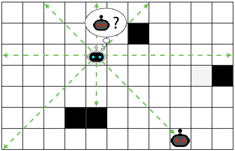
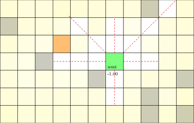
POMDP Example: Light-Dark

2. Solving POMDPs with Tree Search

Solving a POMDP

Environment

Belief Updater

True State

\(s = 7\)

Observation \(o = -0.21\)

\(b\)

\[b_t(s) = P\left(s_t = s \mid b_0, a_0, o_1 \ldots a_{t-1}, o_{t}\right)\]

\[ = P\left(s_t = s \mid b_{t-1}, a_{t-1}, o_{t}\right)\]

\(a\)

\[b_{t+1}(s') \propto Z(o \mid a, s')\int_{s \in \mathcal{S}} T(s' \mid s, a) b_t(s) ds\]

\(O(|\mathcal{S}|^2)\) for finite \(\mathcal{S}\)

State

Timestep

POMDP Example: Light-Dark

Solving a POMDP

Environment

Belief Updater

Planner

\(a = +10\)

True State

\(s = 7\)

Observation \(o = -0.21\)

\(b\)

\[b_t(s) = P\left(s_t = s \mid b_0, a_0, o_1 \ldots a_{t-1}, o_{t}\right)\]

\[ = P\left(s_t = s \mid b_{t-1}, a_{t-1}, o_{t}\right)\]

\(Q(b, a)\)

Why are POMDPs difficult?

Curse of History
Curse of dimensionality
1. State space
2. Observation space
3. Action space

Tree size: \(O\left(\left(|A||O|\right)^D\right)\)

Curse of Dimensionality

\(d\) dimensions, \(k\) segments \(\,\rightarrow \, |S| = k^d\)

1 dimension

e.g. \(s = x \in S = \{1,2,3,4,5\}\)

\(|S| = 5\)

2 dimensions

e.g. \(s = (x,y) \in S = \{1,2,3,4,5\}^2\)

\(|S| = 25\)

3 dimensions

e.g. \(s = (x,y,x_h) \in S = \{1,2,3,4,5\}^3\)

\(|S| = 125\)

(Discretize each dimension into 5 segments)

\(x\)

\(y\)

\(x_h\)

3. Breaking the Curse of Dimensionality

Integration

Find \(\underset{s\sim b}{E}[f(s)]\)

\[=\sum_{s \in S} f(s) b(s)\]

Monte Carlo Integration

\(Q_N \equiv \frac{1}{N} \sum_{i=1}^N f(s_i)\)

\(s_i \sim b\) i.i.d.

\(\text{Var}(Q_N) = \text{Var}\left(\frac{1}{N} \sum_{i=1}^N f(s_i)\right)\)

\(= \frac{1}{N^2} \sum_{i=1}^N\text{Var}\left(f(s_i)\right)\)

\(= \frac{1}{N} \text{Var}\left(f(s_i)\right)\)

\[P(|Q_N - E[f(s_i)]| \geq \epsilon) \leq \frac{\text{Var}(f(s_i))}{N \epsilon^2}\]

(Bienayme)

(Chebyshev)

Curse of dimensionality!

Particle Filter POMDP Approximation

\[b(s) \approx \sum_{i=1}^N \delta_{s}(s_i)\; w_i\]

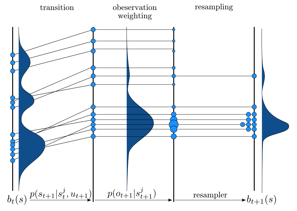
\[b_{t+1}(s') \propto Z(o \mid a, s')\int_{s \in \mathcal{S}} T(s' \mid s, a) b_t(s)\]

\(\implies\) Sample \(s'_i\) from \(T(s' | s_i, a)\),

\(w'_i \propto w_i \times Z(o \mid a, s'_i)\)

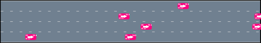
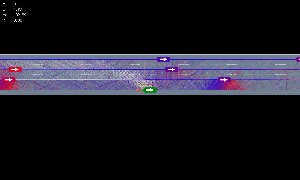
Example: Autonomous Driving

POMDP Formulation

\(s=\left(x, y, \dot{x}, \left\{(x_c,y_c,\dot{x}_c,l_c,\theta_c)\right\}_{c=1}^{n}\right)\)

\(o=\left\{(x_c,y_c,\dot{x}_c,l_c)\right\}_{c=1}^{n}\)

\(a = (\ddot{x}, \dot{y})\), \(\ddot{x} \in \{0, \pm 1 \text{ m/s}^2\}\), \(\dot{y} \in \{0, \pm 0.67 \text{ m/s}\}\)

R(s, a, s') = \text{in\_goal}(s') - \lambda \left(\text{any\_hard\_brakes}(s, s') + \text{any\_too\_slow}(s')\right)

Ego external state

External states of other cars

Internal states of other cars

External states of other cars

Actions shielded (based only on external states) so they can never cause crashes
Braking action always available

Efficiency

Safety

MDP trained on normal drivers

MDP trained on all drivers

Omniscient

POMCPOW (Ours)

Simulation results

[Sunberg & Kochenderfer, T-ITS 2023]

Convergence?

Key 1: Self Normalized Infinite Renyi Divergence Concentation

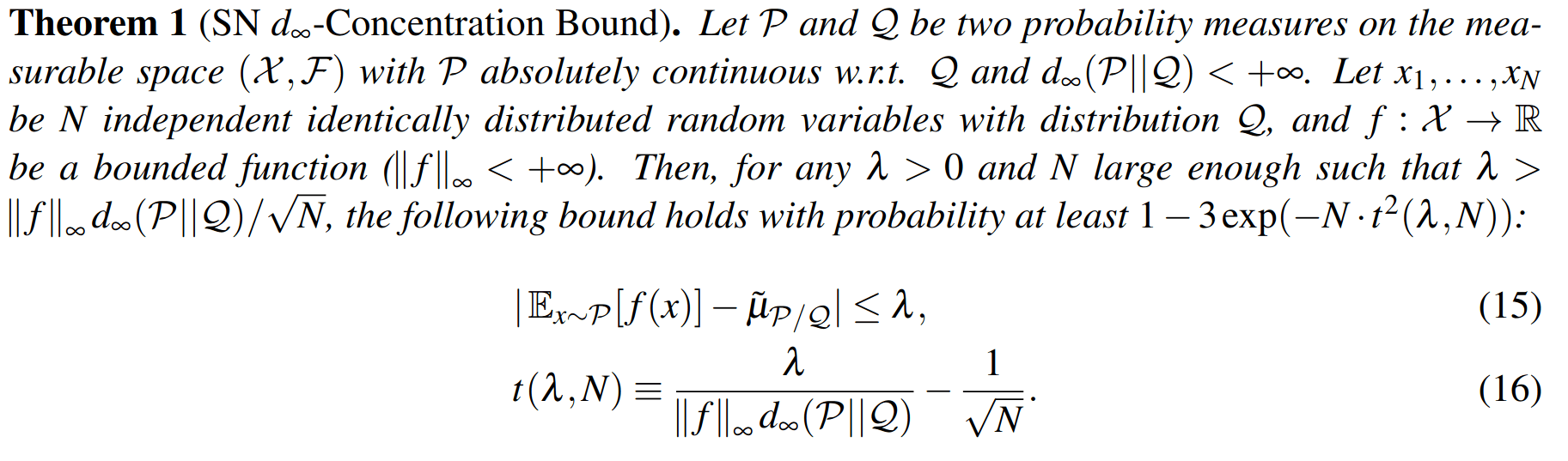
\(\mathcal{P}\): state distribution conditioned on observations (belief)

\(\mathcal{Q}\): marginal state distribution (proposal)

Key 2: Sparse Sampling

Expand for all actions (\(\left|\mathcal{A}\right| = 2\) in this case)

...

Expand for all \(\left|\mathcal{S}\right|\) states

\(C=3\) states

SS-\(\omega\) is close to Belief MDP

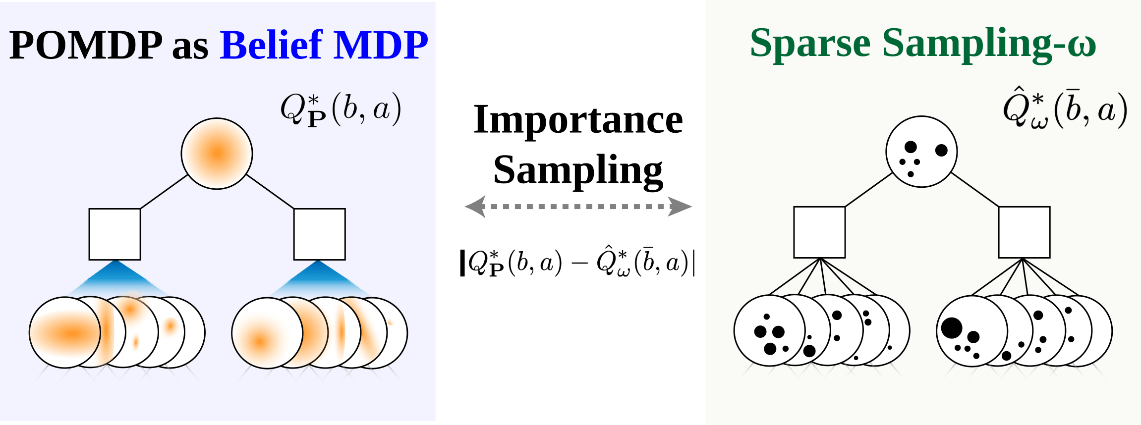
SS-\(\omega\) close to Particle Belief MDP (in terms of Q)

PF Approximation Accuracy

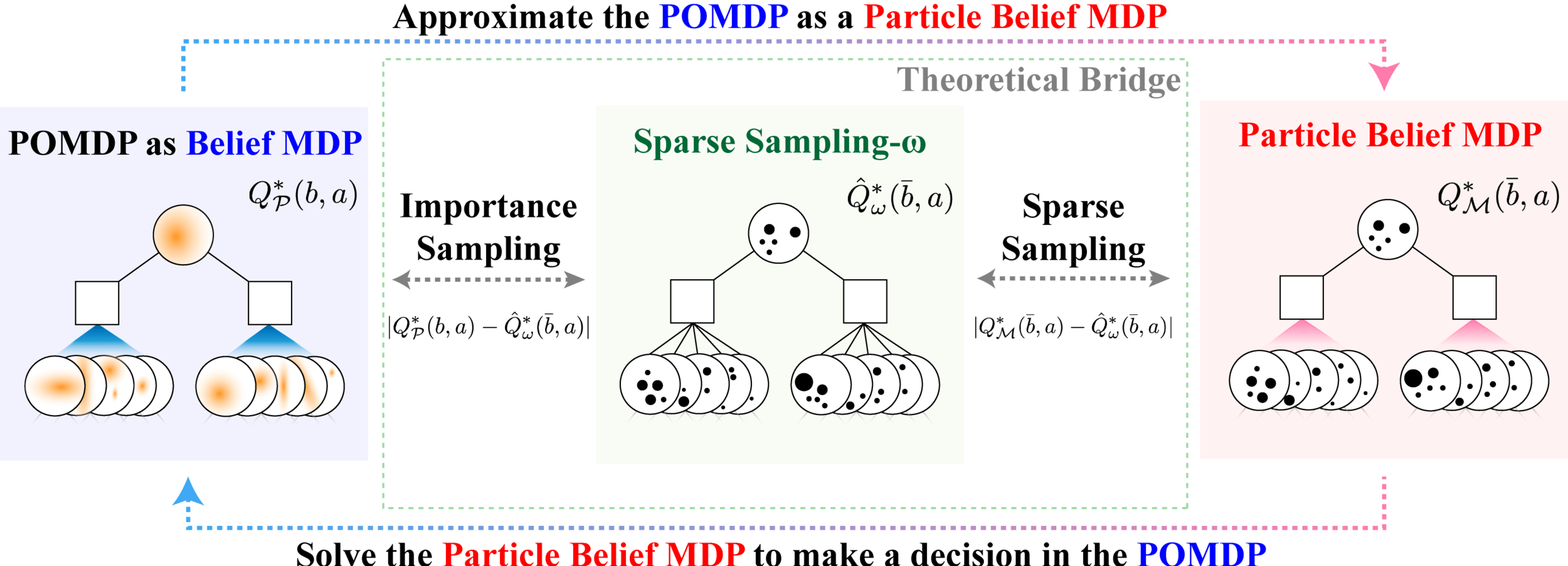
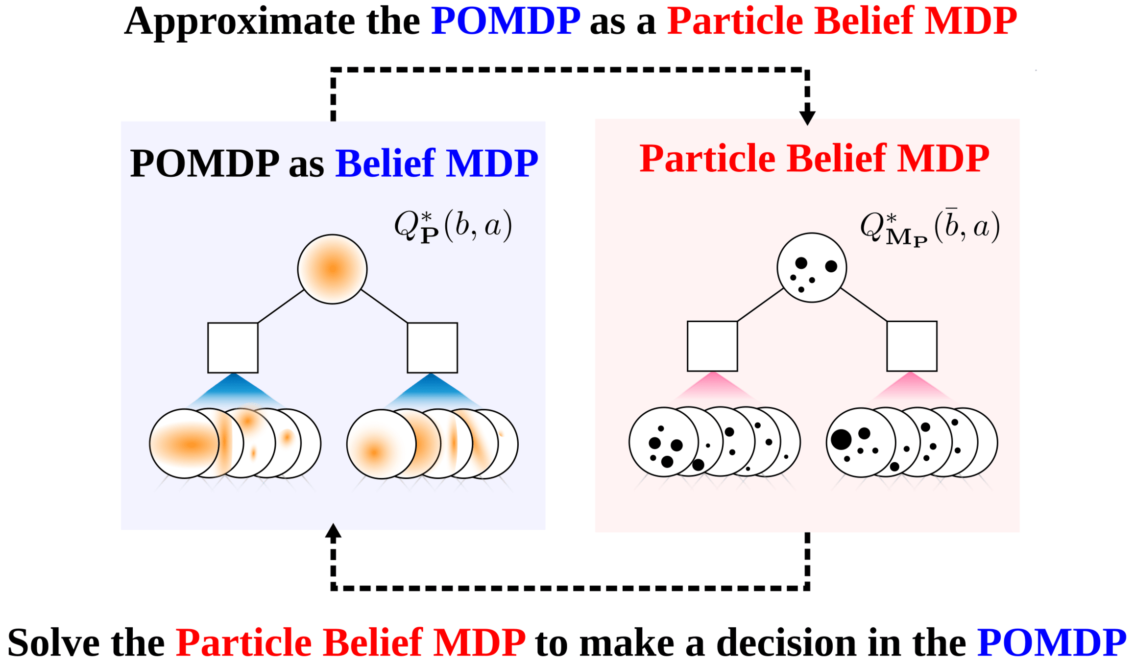
\[|Q_{\mathbf{P}}^*(b,a) - Q_{\mathbf{M}_{\mathbf{P}}}^*(\bar{b},a)| \leq \epsilon \quad \text{w.p. } 1-\delta\]

For any \(\epsilon>0\) and \(\delta>0\), if \(C\) (number of particles) is high enough,

[Lim, Becker, Kochenderfer, Tomlin, & Sunberg, JAIR 2023]

No direct dependence on \(|\mathcal{S}|\) or \(|\mathcal{O}|\)!

Particle belief planning suboptimality

\(C\) is too large for any direct safety guarantees. But, in practice, works extremely well for improving efficiency.

[Lim, Becker, Kochenderfer, Tomlin, & Sunberg, JAIR 2023]

Why are POMDPs difficult?

Curse of History
Curse of dimensionality
1. State space
2. Observation space
3. Action space

Tree size: \(O\left(\left(|A|C\right)^D\right)\)

Solve simplified surrogate problem for policy deep in the tree

[Lim, Tomlin, and Sunberg, 2021]

Takeaways

POMDPs:
- If you have enough knowledge (e.g. sampleable T and explicit Z), solve as a particle belief MDP
- Don't worry too much about the curse of dimensionality in the state or observation space (Sparse sampling + particle filtering will help it)
POSGs:
- Belief-based approaches are a losing battle
- One approach is CDIT - unifies particle-filtering POMDP methods

4. Partially observable stochastic games (POSGs)

POMDP Planning with Learned Components

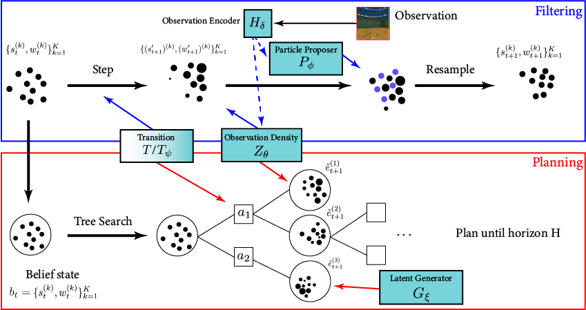
[Deglurkar, Lim, Sunberg, & Tomlin, 2023]