Safe and efficient autonomy in the face of uncertainty
or How I stopped worrying about the curse of dimensionality
Professor Zachary Sunberg
University of Colorado Boulder
Fall 2022
Presentation Map:
- Safety, Efficiency, and Uncertainty
- Online Tree Search in POMDPs
- Incomplete Information Games in Space Domain Awareness
- Open-source Software
Mission: deploy autonomy with confidence

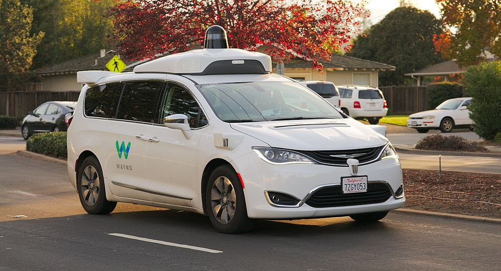
Waymo Image By Dllu - Own work, CC BY-SA 4.0, https://commons.wikimedia.org/w/index.php?curid=64517567

Two Objectives for Autonomy
EFFICIENCY
SAFETY
Minimize resource use
(especially time)
Minimize the risk of harm to oneself and others
Safety often opposes Efficiency
Tweet by Nitin Gupta
29 April 2018
https://twitter.com/nitguptaa/status/990683818825736192
Pareto Optimization
Safety
Better Performance
Model \(M_2\), Algorithm \(A_2\)
Model \(M_1\), Algorithm \(A_1\)
Efficiency
$$\underset{\pi}{\mathop{\text{maximize}}} \, V^\pi = V^\pi_\text{E} + \lambda V^\pi_\text{S}$$
Safety
Weight
Efficiency
Safety, Efficiency, and Uncertainty: A Story
Safety, Efficiency, and Uncertainty: A Story
Why?
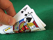
Only one safety procedure: Don't approach the vehicle for 10 minutes after a crash (in case it explodes)
Efficiency: Fly planes
Safety: Avoid fires
Solution: gather information (reduce uncertainty) about potentially unsafe situations
Types of Uncertainty
Alleatory
Epistemic (Static)
Epistemic (Dynamic)


Interaction
MDP
RL
POMDP
Game
Markov Decision Process (MDP)
- \(\mathcal{S}\) - State space
- \(T:\mathcal{S}\times \mathcal{A} \times\mathcal{S} \to \mathbb{R}\) - Transition probability distribution
- \(\mathcal{A}\) - Action space
- \(R:\mathcal{S}\times \mathcal{A} \to \mathbb{R}\) - Reward

Alleatory
Reinforcement Learning
- \(\mathcal{S}\) - State space
- \(T:\mathcal{S}\times \mathcal{A} \times\mathcal{S} \to \mathbb{R}\) - Transition probability distribution
- \(\mathcal{A}\) - Action space
- \(R:\mathcal{S}\times \mathcal{A} \to \mathbb{R}\) - Reward
Alleatory
Epistemic (Static)
Partially Observable Markov Decision Process (POMDP)

- \(\mathcal{S}\) - State space
- \(T:\mathcal{S}\times \mathcal{A} \times\mathcal{S} \to \mathbb{R}\) - Transition probability distribution
- \(\mathcal{A}\) - Action space
- \(R:\mathcal{S}\times \mathcal{A} \to \mathbb{R}\) - Reward
- \(\mathcal{O}\) - Observation space
- \(Z:\mathcal{S} \times \mathcal{A}\times \mathcal{S} \times \mathcal{O} \to \mathbb{R}\) - Observation probability distribution
Alleatory
Epistemic (Static)
Epistemic (Dynamic)
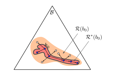
Incomplete Information Game
Alleatory
Epistemic (Static)
Epistemic (Dynamic)
Interaction

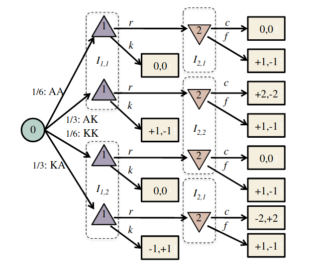
- Finite set of \(n\) players, plus the "chance" player
- \(P(h)\) (player at each history)
- \(A(h)\) (set of actions at each history)
- \(I(h)\) (information set that each history maps to)
- \(U(h)\) (payoff for each leaf node in the game tree)
Image from Russel and Norvig
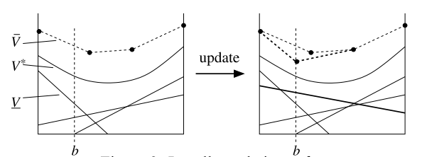
Solving MDPs - The Value Function
$$V^*(s) = \underset{a\in\mathcal{A}}{\max} \left\{R(s, a) + \gamma E\Big[V^*\left(s_{t+1}\right) \mid s_t=s, a_t=a\Big]\right\}$$
Involves all future time
Involves only \(t\) and \(t+1\)
$$\underset{\pi:\, \mathcal{S}\to\mathcal{A}}{\mathop{\text{maximize}}} \, V^\pi(s) = E\left[\sum_{t=0}^{\infty} \gamma^t R(s_t, \pi(s_t)) \bigm| s_0 = s \right]$$
$$Q(s,a) = R(s, a) + \gamma E\Big[V^* (s_{t+1}) \mid s_t = s, a_t=a\Big]$$
Value = expected sum of future rewards
Challenge: Curse of dimensionality
MDP
POMDP
Inc. Info. Game
Curse of Dimensionality
Immediate Reward: \(R(s, a)\)
Value Function: \[Q(s, a) = \text{E}\left[\sum_{t=0}^\infty R(s_t, a_t)\right]\]
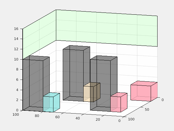
\(d\) dimensions, \(k\) segments \(\,\rightarrow \, |S| = k^d\)
Curse of Dimensionality
\(d\) dimensions, \(k\) segments \(\,\rightarrow \, |\mathcal{S}| = k^d\)


1 dimension, 5 segments
\(|\mathcal{S}| = 5\)
2 dimensions, 5 segments
\(|\mathcal{S}| = 25\)
3 dimensions, 5 segments
\(|\mathcal{S}| = 125\)
Challenge: Curse of dimensionality
Adopted Solution: Online sparse tree search
MDP
POMDP
Inc. Info. Game
Online Tree Search in MDPs

Time
Estimate \(Q(s, a)\) based on children
Sparse Sampling
Expand for all actions (\(\left|\mathcal{A}\right| = 2\) in this case)
...
Expand for all \(\left|\mathcal{S}\right|\) states
\(C=3\) states
Sparse Sampling
...
[Kearns, Mansour, & Ng, 2002]
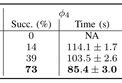
1. Near-optimal policy: \(\left|V^\text{SS}(s) - V^*(s) \right|\leq \epsilon\)
2. Running time independent of state space size:
\(O \left( ( \left|\mathcal{A} \right|C )^H \right) \)
Challenge: Curse of dimensionality
Adopted Solution: Online sparse tree search
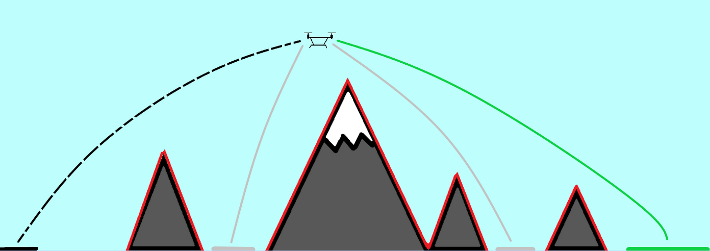
Shortcoming: No active information gathering
Additional Challenge: Curse of history
MDP
POMDP
Inc. Info. Game

State
Timestep
Accurate Observations
Goal: \(a=0\) at \(s=0\)
Optimal Policy
Localize
\(a=0\)
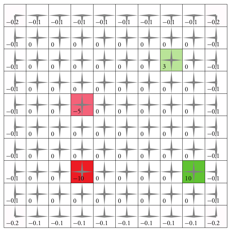
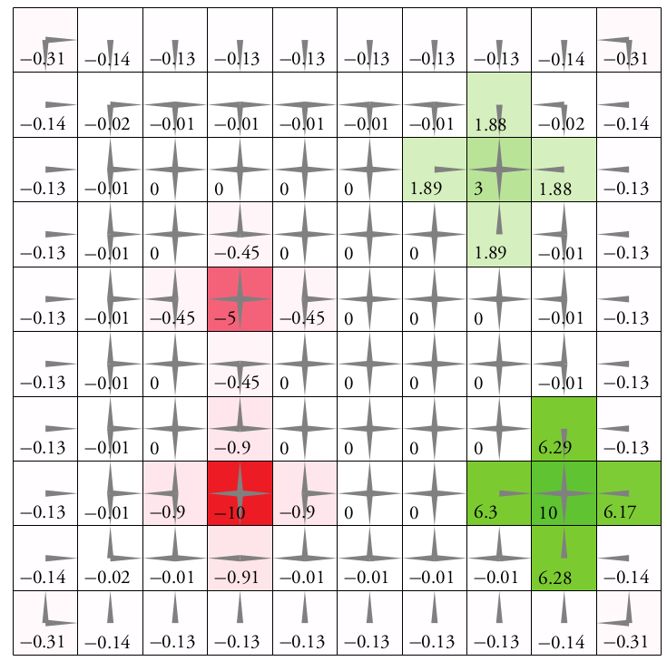
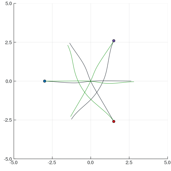
POMDP Example: Light-Dark
POMDP Sense-Plan-Act Loop
Environment
Belief Updater
Policy/Planner
\(b\)
\(a\)
\[b_t(s) = P\left(s_t = s \mid a_1, o_1 \ldots a_{t-1}, o_{t-1}\right)\]

True State
\(s = 7\)
Observation \(o = -0.21\)
\(O(S^2)\)
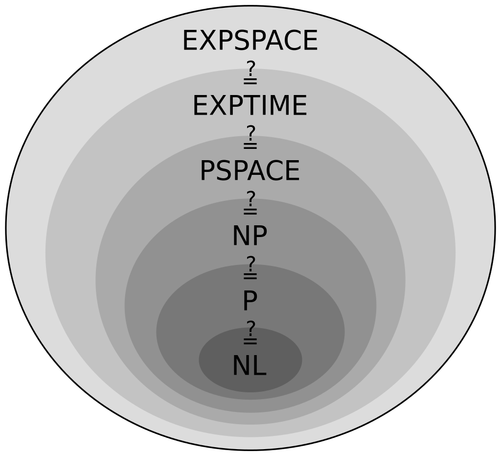
A POMDP is an MDP on the Belief Space
SARSOP can solve some POMDPs with thousands of states offline
but
The POMDP is PSPACE-Complete
Intractable!
- A POMDP is an MDP on the Belief Space but belief updates are expensive
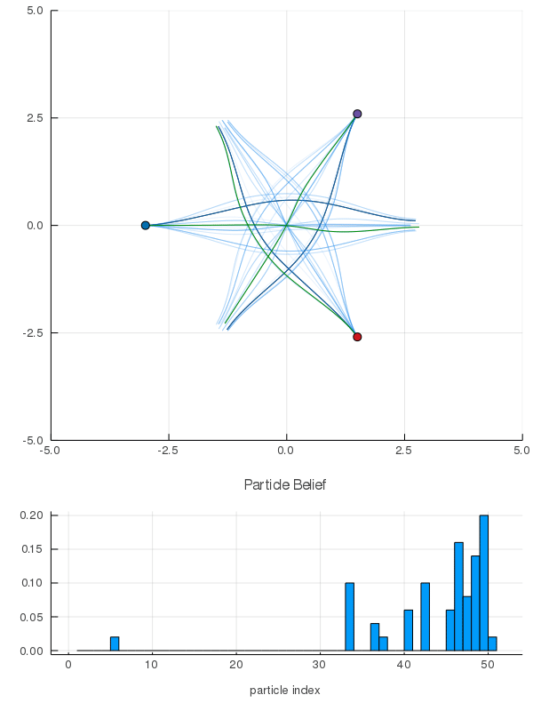
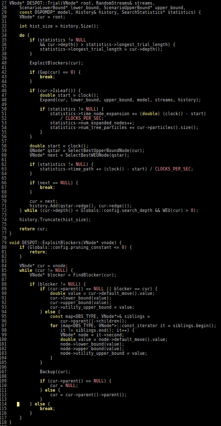
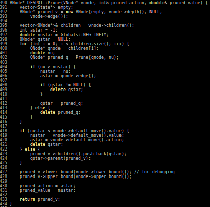
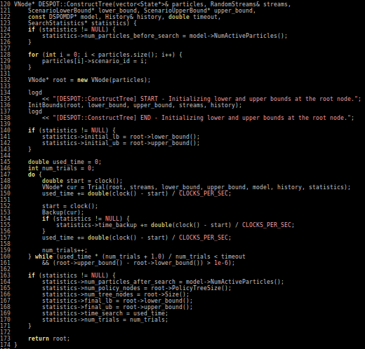
- POMCP* uses simulations of histories instead of full belief updates
- Each belief is implicitly represented by a collection of unweighted particles


[Ross, 2008] [Silver, 2010]
*(Partially Observable Monte Carlo Planning)
REVISE SLIDE FOR FUTURE


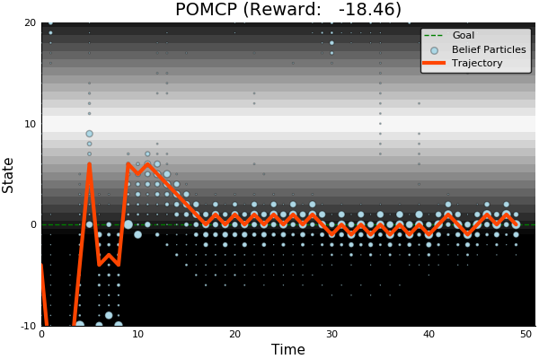
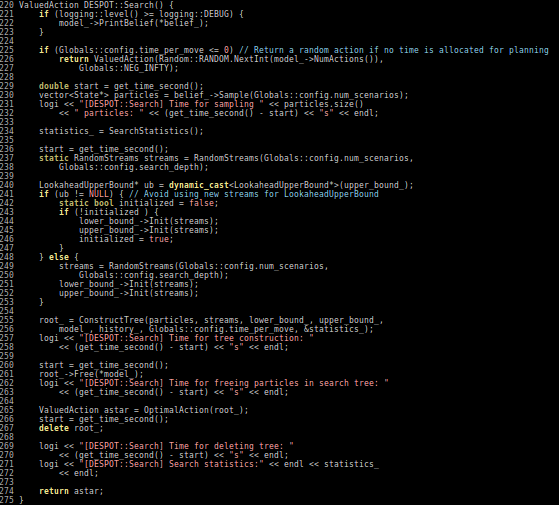
POMCP
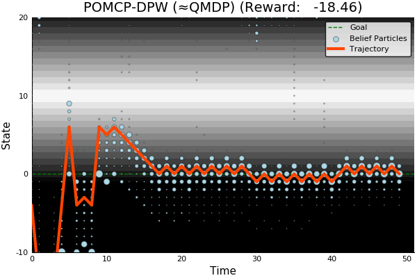
POMCP-DPW
POMCPOW
[Sunberg and Kochenderfer, ICAPS 2018]
First scalable algorithm for general POMDPs with continuous \(O\)
REMOVE SLIDE IN FUTURE
Challenge: Curse of dimensionality
Adopted Solution: Online sparse tree search
Shortcoming: No active information gathering
Additional Challenge: Curse of history
Adopted Solution: Particle filtering
MDP
POMDP
Inc. Info. Game
POMDP = Belief MDP
PF Approximation Accuracy
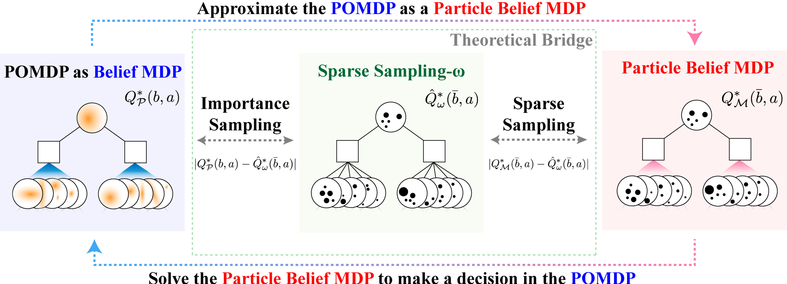
\[|Q_{\mathbf{P}}^*(b,a) - Q_{\mathbf{M}_{\mathbf{P}}}^*(\bar{b},a)| \leq \epsilon \quad \text{w.p. } 1-\delta\]
For and \(\epsilon>0\) and \(\delta>0\), if \(C\) (number of particles) is high enough,
\(\mathbf{M}_\mathbf{P}\) = Particle belief MDP approximation of POMDP \(\mathbf{P}\)
[Lim, Becker, Kochenderfer, Tomlin, & Sunberg, 2022]
No dependence on \(|\mathcal{S}|\) or \(\mathcal{O}\)!
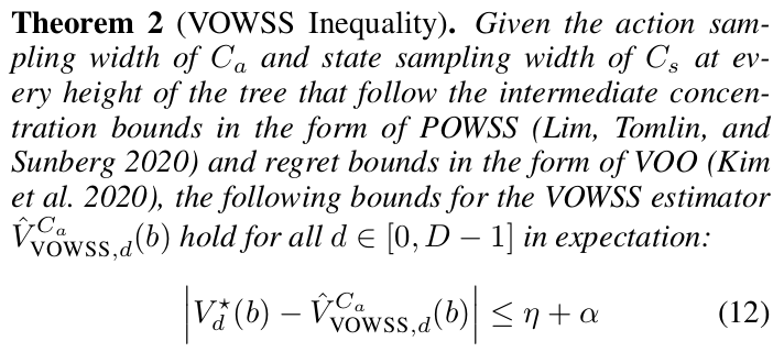
Continuous Observation Analytical Results (POWSS)
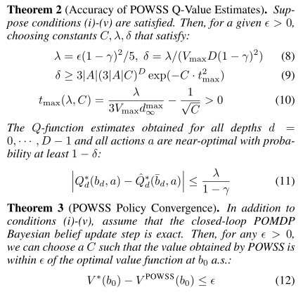
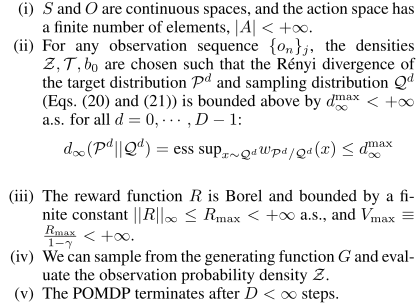
Our simplified algorithm is near-optimal
[Lim, Tomlin, & Sunberg, IJCAI 2020]
Easy MDP to POMDP Extension

Is POMDP Planning worth the computational effort in realistic scenarios?
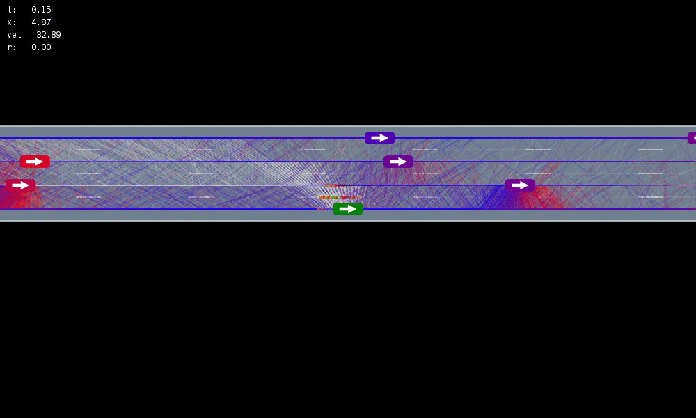


MDP trained on normal drivers


MDP trained on all drivers
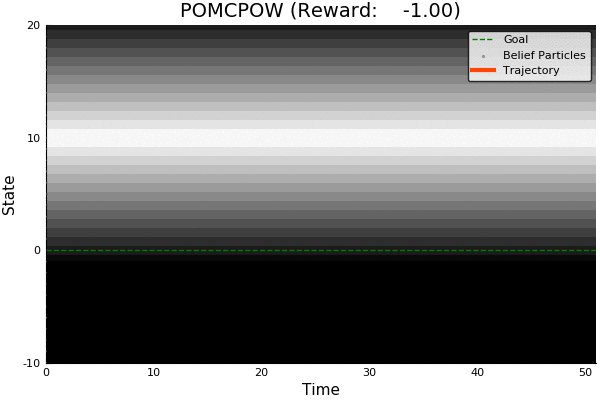
Omniscient
POMCPOW (Ours)
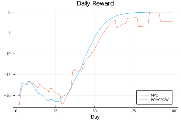
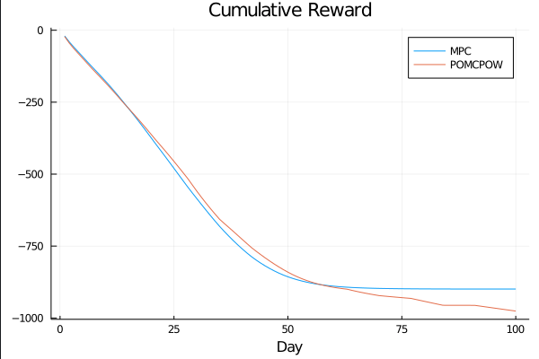
Simulation results
[Sunberg & Kochenderfer, T-ITS 2022]

Conventional 1D POMDP
2D POMDP
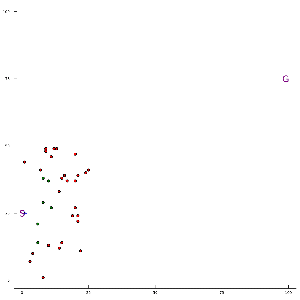
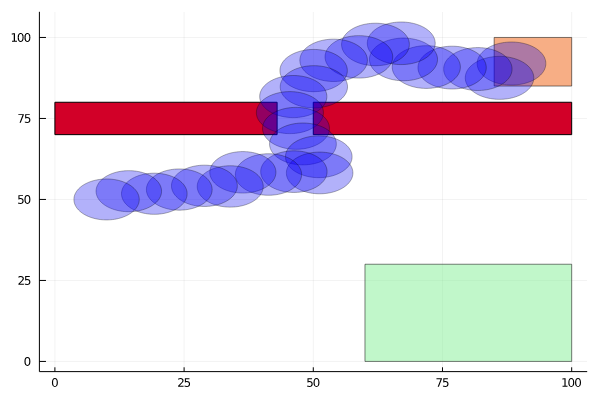
Pedestrian Navigation
[Gupta, Hayes, & Sunberg, AAAI 2021]
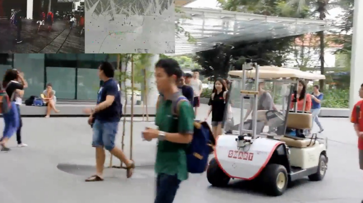
POMDP Planning with Image Observations
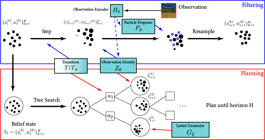
[Deglurkar, Lim, Sunberg, & Tomlin, 2023?]
Actions
Observations
States
POMDPs with Continuous...
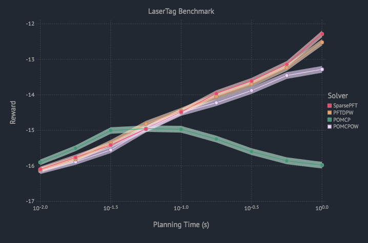
- PO-UCT (POMCP)
- DESPOT
- POMCPOW
- DESPOT-α
- LABECOP
- Ada-OPS
- GPS-ABT
- BOMCP
- VOMCPOW
BOMCP


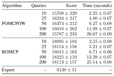
[Mern, Sunberg, et al. AAAI 2021]
Voronoi Progressive Widening
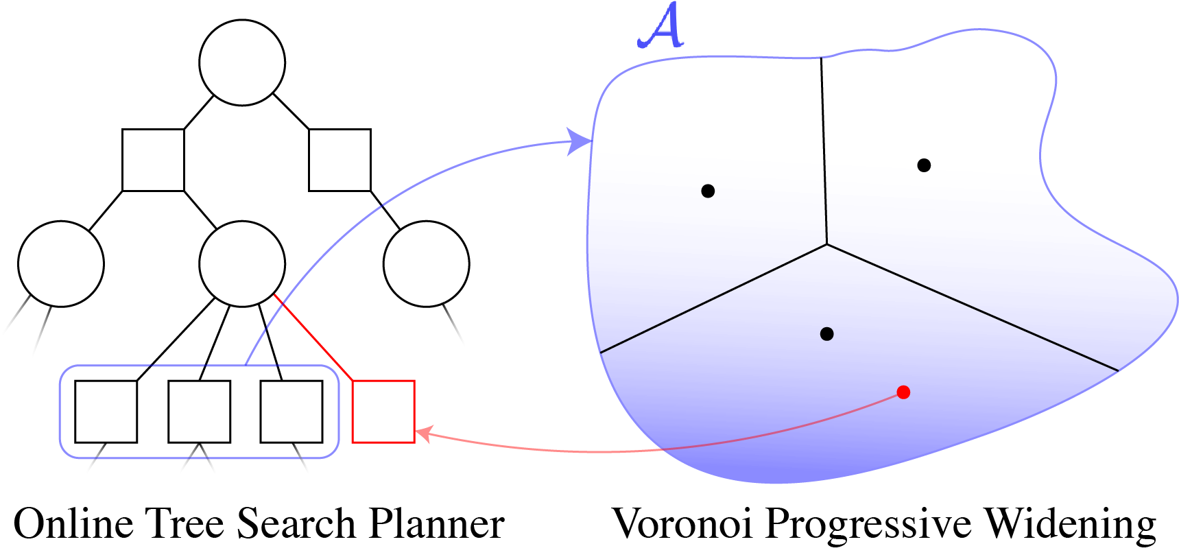
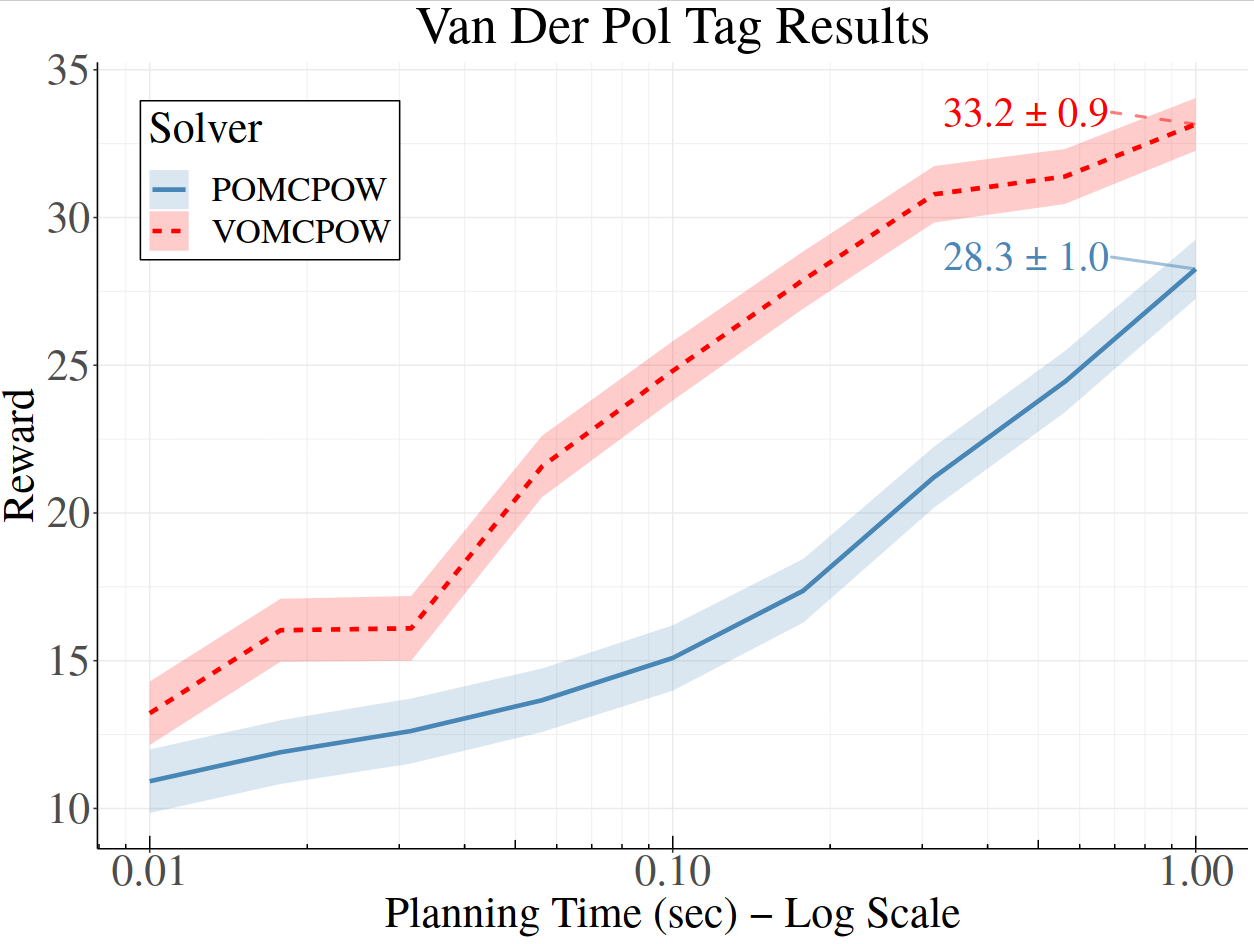
[Lim, Tomlin, & Sunberg CDC 2021]
Motion Planning under Uncertainty with Temporal Logic Specifications
[Ho, Sunberg, and Lahijanian, ICRA 2022, ICRA 2023 (?)]
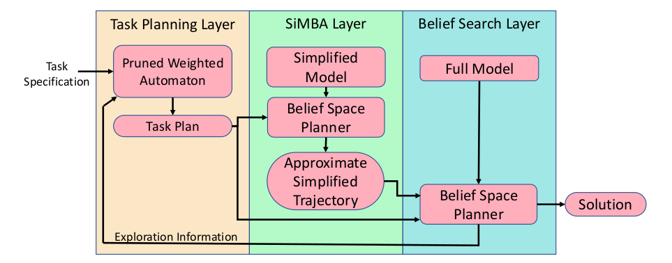
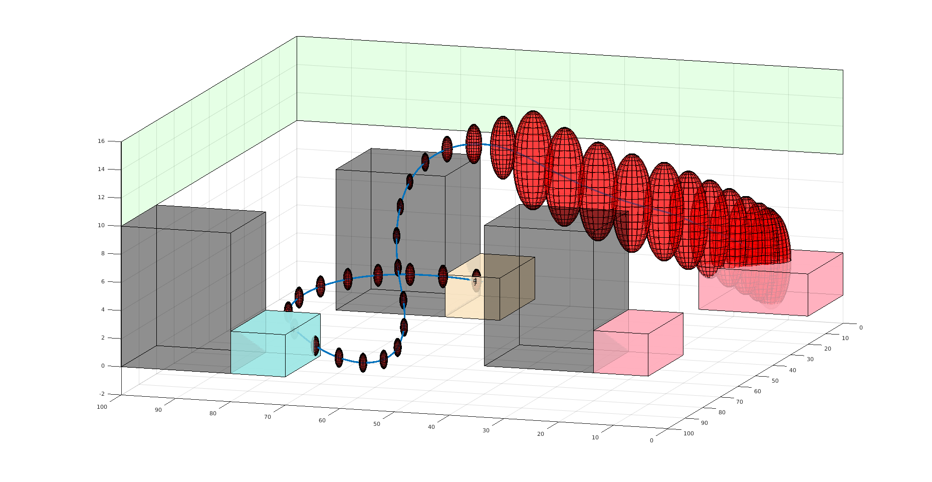
Key Idea: Simplified Model with Belief Approximation (SiMBA)
Challenge: Curse of dimensionality
Adopted Solution: Online sparse tree search
Shortcoming: No active information gathering
Additional Challenge: Curse of history
Adopted Solution: Particle filtering
Shortcoming: No mixed strategies
MDP
POMDP
Inc. Info. Game
POMDP = Belief MDP
Interaction Uncertainty


[Peters, Tomlin, and Sunberg 2020]
Game Theory
Nash Equilibrium: All players play a best response.
Optimization Problem
(MDP or POMDP)
\(\text{maximize} \quad f(x)\)
Game
Player 1: \(U_1 (a_1, a_2)\)
Player 2: \(U_2 (a_1, a_2)\)
Collision
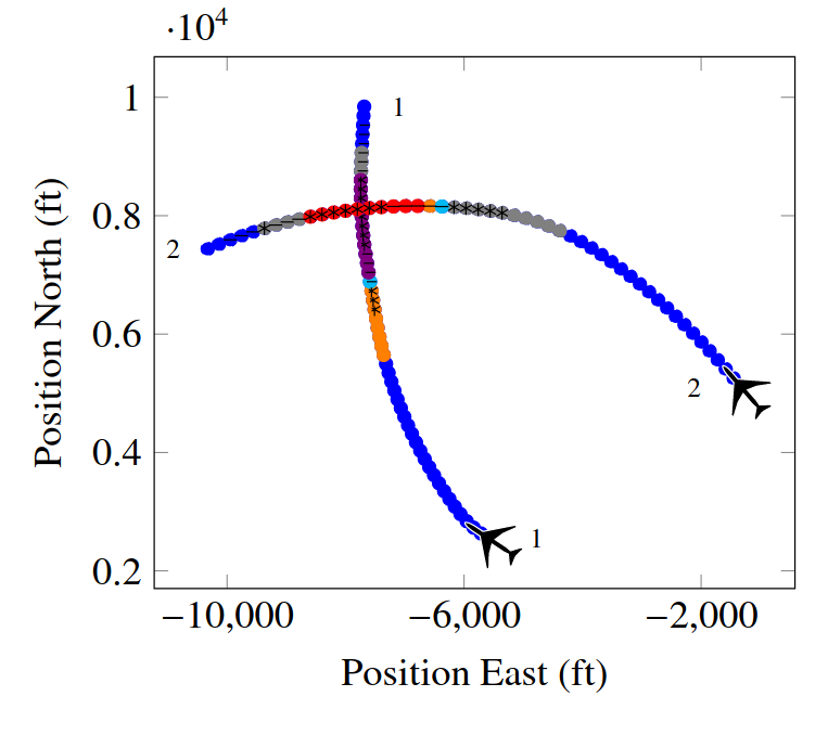
Example: Airborne Collision Avoidance
|
|
|
|
|
Player 1
Player 2
Up
Down
Up
Down
-6, -6
-1, 1
1, -1
-4, -4

Collision
Mixed Strategies
Nash Equilibrium \(\iff\) Zero Exploitability
\[\sum_i \max_{\pi_i'} U_i(\pi_i', \pi_{-i})\]
No Pure Nash Equilibrium!
Instead, there is a Mixed Nash where each player plays up or down with 50% probability.
If either player plays up or down more than 50% of the time, their strategy can be exploited.
Exploitability (zero sum):
Strategy (\(\pi_i\)): probability distribution over actions
|
|
|
|
|
Up
Down
Up
Down
-1, 1
1, -1
1, -1
-1, 1
Collision
Collision


Challenge: Curse of dimensionality
Adopted Solution: Online sparse tree search
Shortcoming: No active information gathering
Additional Challenge: Curse of history
Adopted Solution: Particle filtering
Shortcoming: No mixed strategies
MDP
POMDP
Inc. Info. Game
Additional Challenge: Computing Mixed strategies
Solution: ???
POMDP = Belief MDP
Best response = POMDP
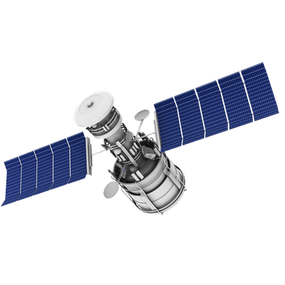
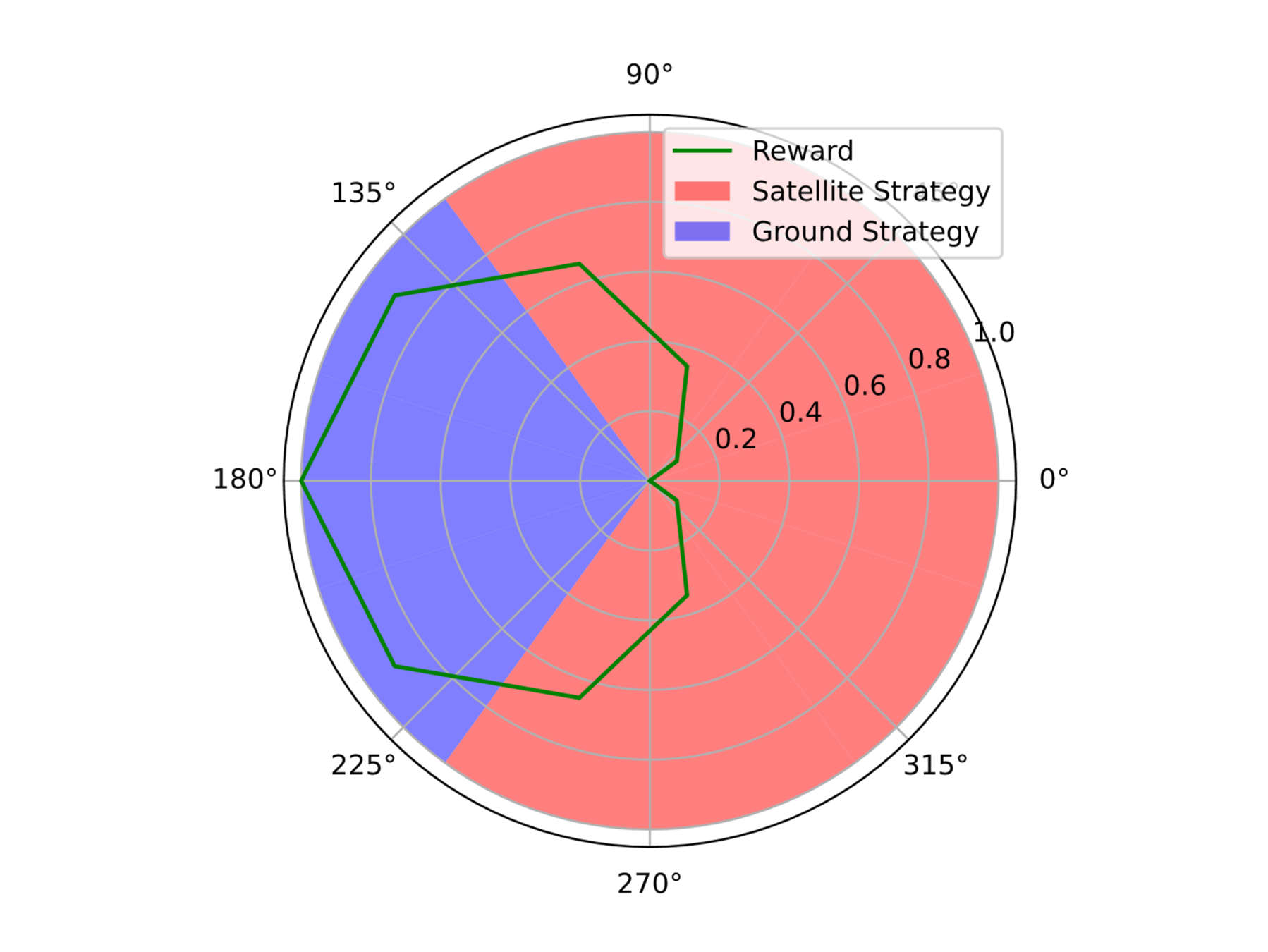
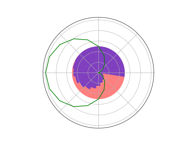
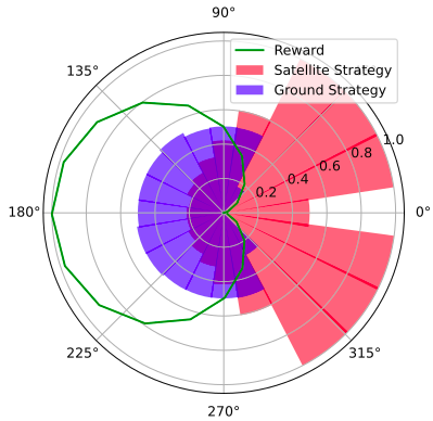
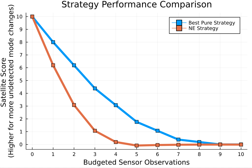
Space Domain Awareness Games
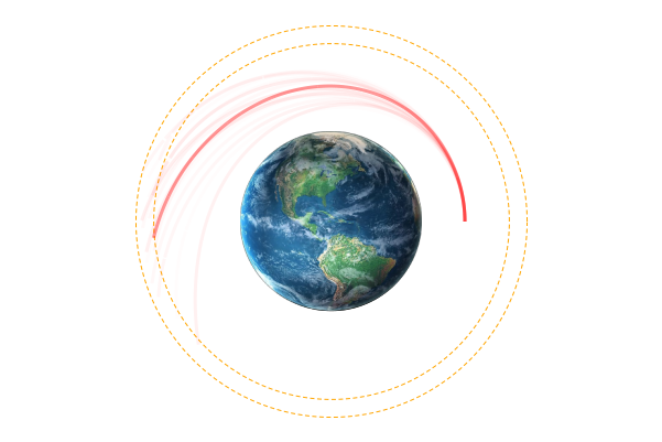
Simplified SDA Game

1
2
...
...
...
...
...
...
...
\(N\)
[Becker & Sunberg CDC 2021]
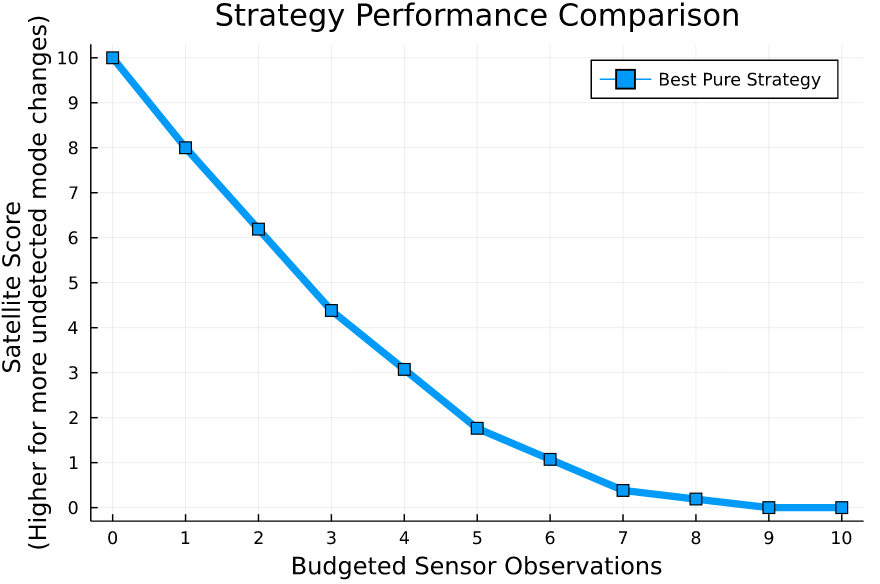
Counterfactual Regret Minimization Training
Open Source Research Software
Good Examples
- Open AI Gym interface
- OMPL
- ROS
Challenges for POMDP Software
- There is a huge variety of
- Problems
- Continuous/Discrete
- Fully/Partially Observable
- Generative/Explicit
- Simple/Complex
- Solvers
- Online/Offline
- Alpha Vector/Graph/Tree
- Exact/Approximate
- Domain-specific heuristics
- Problems
- POMDPs are computationally difficult.
Explicit
Black Box
("Generative" in POMDP lit.)

\(s,a\)
\(s', o, r\)
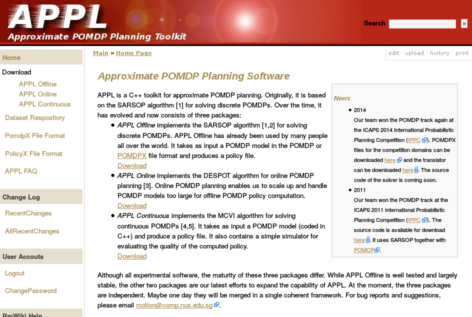
Previous C++ framework: APPL
"At the moment, the three packages are independent. Maybe one day they will be merged in a single coherent framework."
Open Source Research Software
- Performant
- Flexible and Composable
- Free and Open
- Easy for a wide range of people to use (for homework)
- Easy for a wide range of people to understand
C++
Python, C++
Python, Matlab
Python, Matlab
Python, C++
2013

We love [Matlab, Lisp, Python, Ruby, Perl, Mathematica, and C]; they are wonderful and powerful. For the work we do — scientific computing, machine learning, data mining, large-scale linear algebra, distributed and parallel computing — each one is perfect for some aspects of the work and terrible for others. Each one is a trade-off.
We are greedy: we want more.
2012
Julia - Speed
Celeste Project
1.54 Petaflops

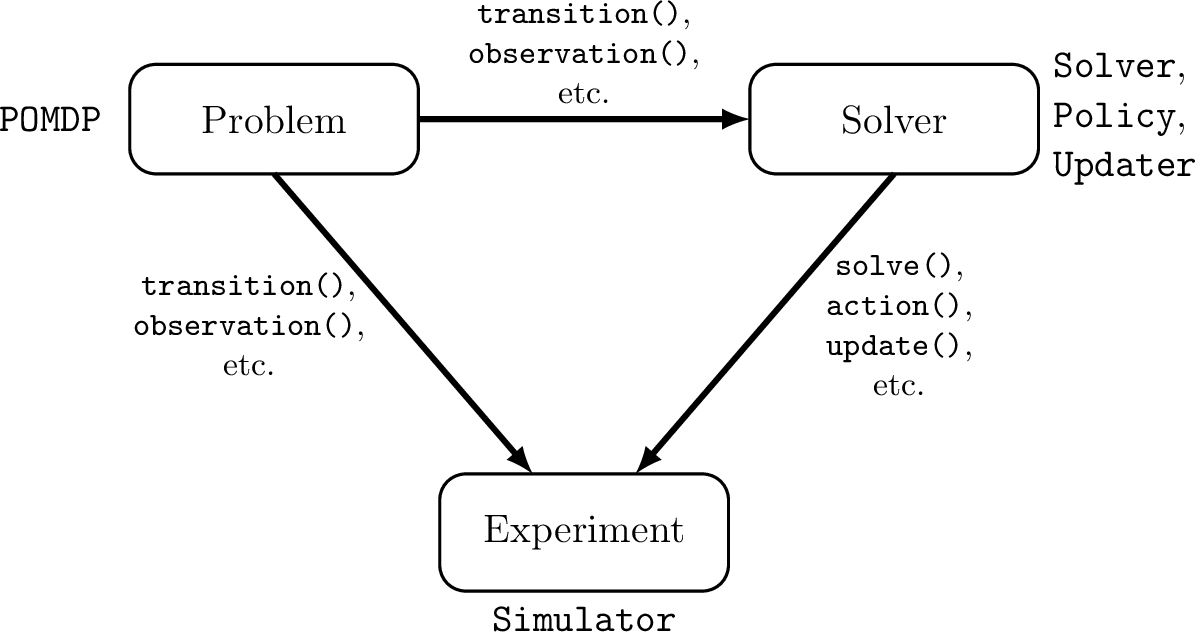
POMDPs.jl - An interface for defining and solving MDPs and POMDPs in Julia

Mountain Car
partially_observable_mountaincar = QuickPOMDP(
    actions = [-1., 0., 1.],
    obstype = Float64,
    discount = 0.95,
    initialstate = ImplicitDistribution(rng -> (-0.2*rand(rng), 0.0)),
    isterminal = s -> s[1] > 0.5,

    gen = function (s, a, rng)
        x, v = s
        vp = clamp(v + a*0.001 + cos(3*x)*-0.0025, -0.07, 0.07)
        xp = x + vp
        if xp > 0.5
            r = 100.0
        else
            r = -1.0
        end
        return (sp=(xp, vp), r=r)
    end,

    observation = (a, sp) -> Normal(sp[1], 0.15)
)
using POMDPs
using QuickPOMDPs
using POMDPPolicies
using Compose
import Cairo
using POMDPGifs
import POMDPModelTools: Deterministic
mountaincar = QuickMDP(
function (s, a, rng)
x, v = s
vp = clamp(v + a*0.001 + cos(3*x)*-0.0025, -0.07, 0.07)
xp = x + vp
if xp > 0.5
r = 100.0
else
r = -1.0
end
return (sp=(xp, vp), r=r)
end,
actions = [-1., 0., 1.],
initialstate = Deterministic((-0.5, 0.0)),
discount = 0.95,
isterminal = s -> s[1] > 0.5,
render = function (step)
cx = step.s[1]
cy = 0.45*sin(3*cx)+0.5
car = (context(), circle(cx, cy+0.035, 0.035), fill("blue"))
track = (context(), line([(x, 0.45*sin(3*x)+0.5) for x in -1.2:0.01:0.6]), stroke("black"))
goal = (context(), star(0.5, 1.0, -0.035, 5), fill("gold"), stroke("black"))
bg = (context(), rectangle(), fill("white"))
ctx = context(0.7, 0.05, 0.6, 0.9, mirror=Mirror(0, 0, 0.5))
return compose(context(), (ctx, car, track, goal), bg)
end
)
energize = FunctionPolicy(s->s[2] < 0.0 ? -1.0 : 1.0)
makegif(mountaincar, energize; filename="out.gif", fps=20)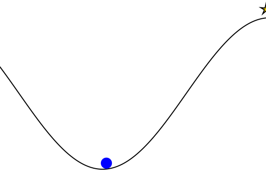


Group


- Astrodynamics
- Autonomous Systems (me)
- Bioastronautics
- Fluids, Structures and Materials
- Remote Sensing
-
Application Deadlines
Spring 2023: October 1
Fall 2023: December 1 -
Applicant Mentoring program
Thank You!

Recent and Current Projects
Human Behavior Model: IDM and MOBIL

M. Treiber, et al., “Congested traffic states in empirical observations and microscopic simulations,” Physical Review E, vol. 62, no. 2 (2000).
A. Kesting, et al., “General lane-changing model MOBIL for car-following models,” Transportation Research Record, vol. 1999 (2007).
A. Kesting, et al., "Agents for Traffic Simulation." Multi-Agent Systems: Simulation and Applications. CRC Press (2009).


All drivers normal


Omniscient
Mean MPC
QMDP
POMCPOW
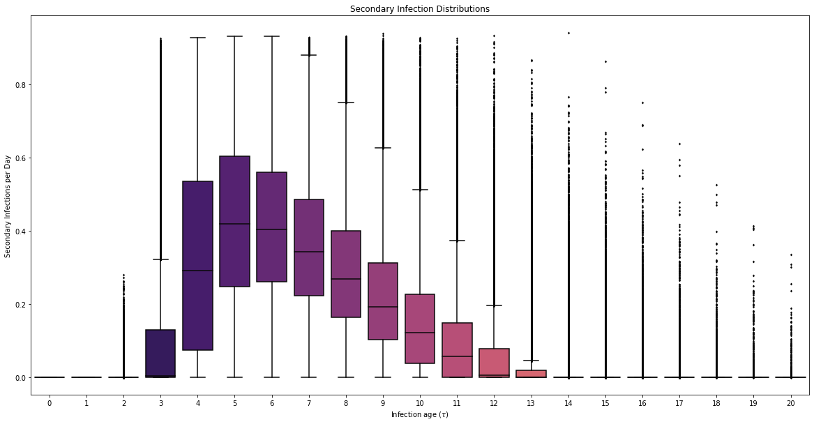
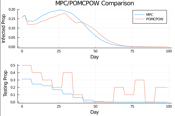
COVID POMDP
Individual Infectiousness
Infection Age
Incident Infections
Need
Test sensitivity is secondary to frequency and turnaround time for COVID-19 surveillance
Larremore et al.
Viral load represented by piecewise-linear hinge function
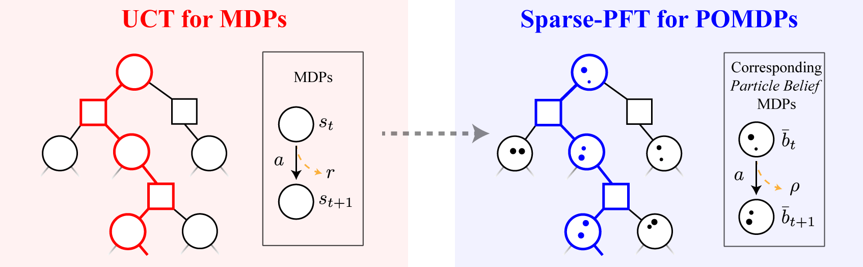
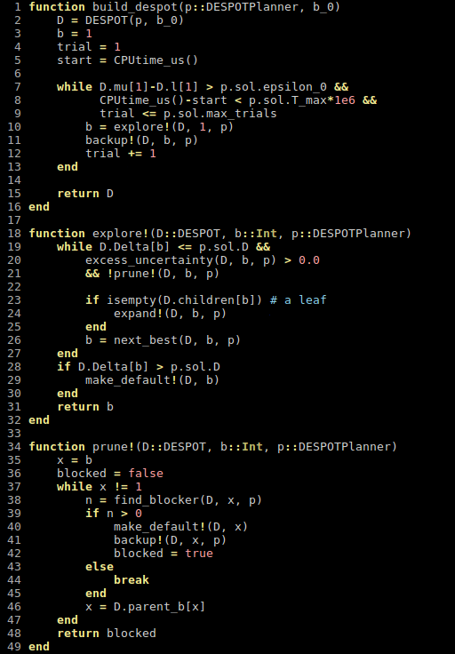
Sparse PFT
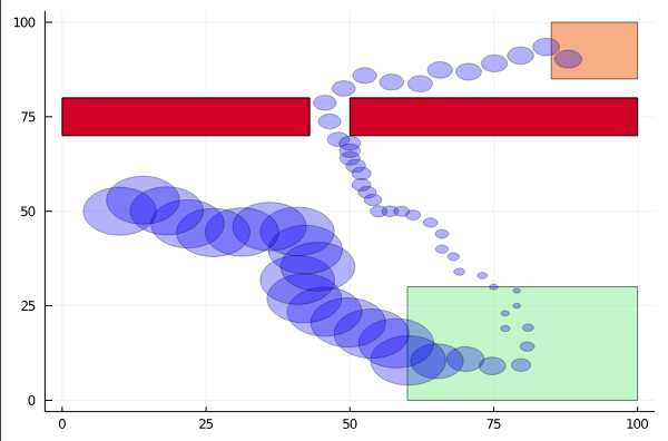
Active Information Gathering for Safety

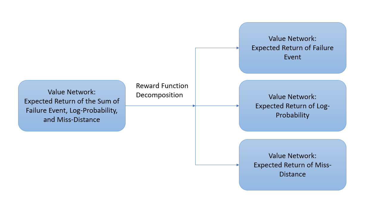
Reward Decomposition for Adaptive Stress Testing


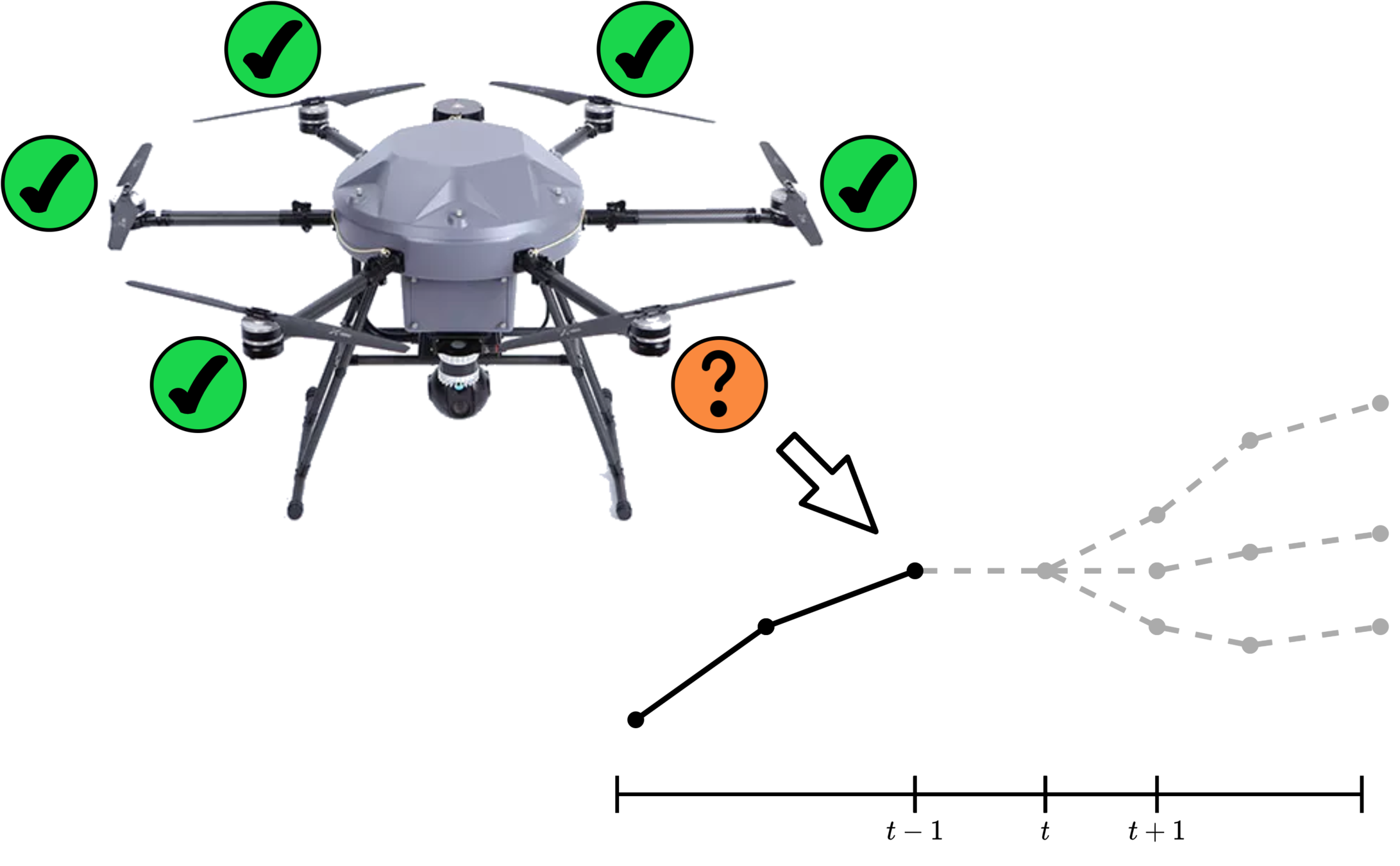
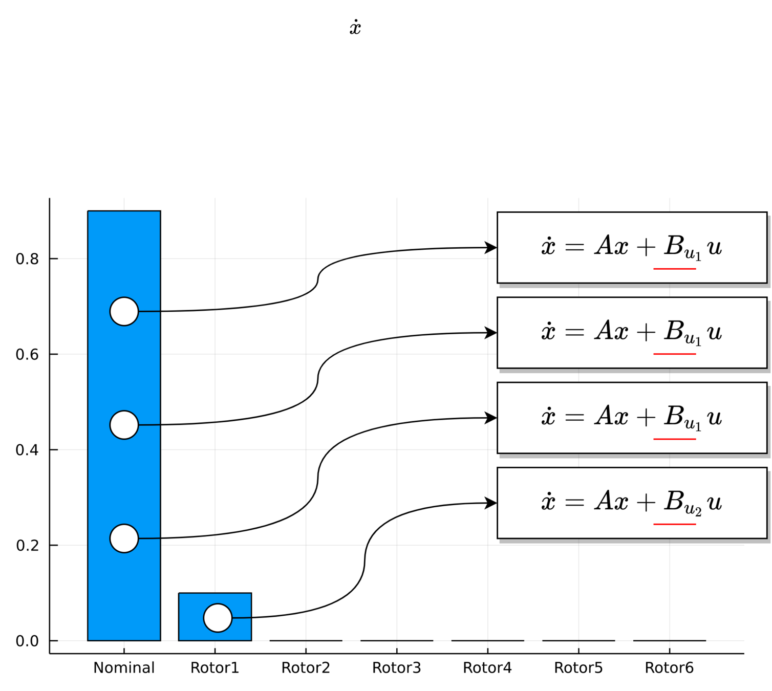
UAV Component Failures
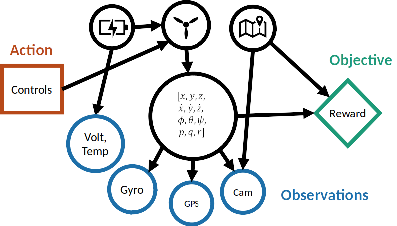
MPC for Intermittent Rotor Failures