POMDPs
Approximations and when they are useful
Outline
- Review Preliminaries
- Approximations
- When is it actually worth it to attempt to solve a POMDP?

Markov Model
- \(\mathcal{S}\) - State space
- \(T:\mathcal{S}\times\mathcal{S} \to \mathbb{R}\) - Transition probability distributions
Markov Decision Process (MDP)
- \(\mathcal{S}\) - State space
- \(T:\mathcal{S}\times \mathcal{A} \times\mathcal{S} \to \mathbb{R}\) - Transition probability distribution
- \(\mathcal{A}\) - Action space
- \(R:\mathcal{S}\times \mathcal{A} \to \mathbb{R}\) - Reward

Solving MDPs - The Value Function
$$V^*(s) = \underset{a\in\mathcal{A}}{\max} \left\{R(s, a) + \gamma E\Big[V^*\left(s_{t+1}\right) \mid s_t=s, a_t=a\Big]\right\}$$
Involves all future time
Involves only \(t\) and \(t+1\)
$$\underset{\pi:\, \mathcal{S}\to\mathcal{A}}{\mathop{\text{maximize}}} \, V^\pi(s) = E\left[\sum_{t=0}^{\infty} \gamma^t R(s_t, \pi(s_t)) \bigm| s_0 = s \right]$$
$$Q(s,a) = R(s, a) + \gamma E\Big[V^* (s_{t+1}) \mid s_t = s, a_t=a\Big]$$
Value = expected sum of future rewards
Online Decision Process Tree Approaches

Time
Estimate \(Q(s, a)\) based on children
$$Q(s,a) = R(s, a) + \gamma E\Big[V^* (s_{t+1}) \mid s_t = s, a_t=a\Big]$$
\[V(s) = \max_a Q(s,a)\]
Partially Observable Markov Decision Process (POMDP)

- \(\mathcal{S}\) - State space
- \(T:\mathcal{S}\times \mathcal{A} \times\mathcal{S} \to \mathbb{R}\) - Transition probability distribution
- \(\mathcal{A}\) - Action space
- \(R:\mathcal{S}\times \mathcal{A} \to \mathbb{R}\) - Reward
- \(\mathcal{O}\) - Observation space
- \(Z:\mathcal{S} \times \mathcal{A}\times \mathcal{S} \times \mathcal{O} \to \mathbb{R}\) - Observation probability distribution
Types of Uncertainty
OUTCOME
MODEL
STATE


Objective Function
$$\underset{\pi}{\mathop{\text{maximize}}} \, E\left[\sum_{t=0}^{\infty} \gamma^t R(s_t, \pi(\cdot)) \right]$$

State
Timestep
Accurate Observations
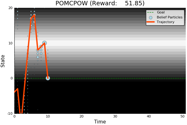
Goal: \(a=0\) at \(s=0\)
Optimal Policy
Localize
\(a=0\)
POMDP Example: Light-Dark
POMDP Sense-Plan-Act Loop
Environment
Belief Updater
Policy
\(h_t = (b_0, a_1, o_1 \ldots a_{t-1}, o_{t-1})\)
\(a\)
\[b_t(s) = P\left(s_t = s \mid h_t \right)\]

True State
\(s = 7\)
Observation \(o = -0.21\)
Environment
Belief Updater
Policy
\(a\)
\(b = \mathcal{N}(\hat{s}, \Sigma)\)
True State
\(s \in \mathbb{R}^n\)
Observation \(o \sim \mathcal{N}(C s, V)\)
LQG Problem (a simple POMDP)
\(s_{t+1} \sim \mathcal{N}(A s_t + B a_t, W)\)
\(\pi(b) = K \hat{s}\)
Kalman Filter
\(R(s, a) = - s^T Q s - a^T R a\)
Belief Updaters
- Discrete Bayes Filter (\(O(|\mathcal{S}|^2)\))
- Kalman Filter
- Particle Filter (\(O(n)\))
- Hybrids: e.g. IMM, Gaussian Mixtures
Belief updates can be used with ANY controller; you don't have to solve a POMDP!
BOARD
C. H. Papadimitriou and J. N. Tsitsiklis, “The complexity of Markov decision processes,” Mathematics of Operations Research, vol. 12, no. 3, pp. 441–450, 1987
Computational Complexity

POMDPs
(PSPACE Complete)
BOARD
Approximations
- Numerical
- Policy information restriction
- Formulation
Numerical Approximations
DESPOT, POMCP, SARSOP, POMCPOW, others
Online, Offline
Goal is to solve the full POMDP approximately
Can find useful approximate solutions to large problems IN REAL TIME
Numerical Approximations
Focus on smaller reachable part of belief space

Policy information restriction
- Certainty equivalent: \(\pi(b) = \pi_s\left(\underset{s\sim b}{E}[s]\right)\)
- Last \(k\) observations

Formulation Approximations
- QMDP
- Fast Informed Bound
- Hindsight Optimization
- Ignore Observations
- Most Likely Observation
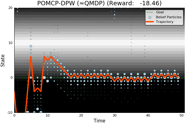
QMDP
POMDP:
QMDP:
\[\pi_{Q_\text{MDP}}(b) = \underset{a\in\mathcal{A}}{\text{argmax}} \underset{s\sim b}{E}\left[Q_\text{MDP}(s,a)\right]\]
where \(Q_\text{MDP}\) are the optimal \(Q\) values for the fully observable MDP. \(O(T |S|^2|A|)\)
$$\pi^* = \underset{\pi: \mathcal{B} \to \mathcal{A}}{\mathop{\text{argmax}}} \, E\left[\sum_{t=0}^{\infty} \gamma^t R(s_t, \pi(b_t)) \right]$$
QMDP

INDUSTRIAL GRADE
QMDP


ACAS X
[Kochenderfer, 2011]
POMDP Solution
QMDP


Same as full observability on the next step
FIB (Fast Informed Bound)

\[\pi_\text{FIB}(b) = \underset{a \in \mathcal{A}}{\text{argmax}}\, \alpha_a^T b\]
- (Sort of) like taking the first observation into account.
- Strictly better value function approximation than QMDP
- \(O(T |S|^2|A||O|)\)
Hindsight Optimization
POMDP:
Hindsight:
$$V_\text{hs}(b) = \underset{s_0 \sim b}{E}\left[\max_{a_t}\sum_{t=0}^{\infty} \gamma^t R(s_t, a_t) \right]$$
$$\pi^* = \underset{\pi: \mathcal{B} \to \mathcal{A}}{\mathop{\text{argmax}}} \, E\left[\sum_{t=0}^{\infty} \gamma^t R(s_t, \pi(b_t)) \right]$$
Ignore Observations
Most Likely Observation
- Replace observation model with most likely given the belief or history
When to try the full POMDP
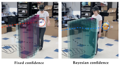
- Costly Information Gathering
- Long-lived uncertainty, consequential actions, and good models
- For comparison with approximations
BOARD
Information Gathering

QMDP
Full POMDP


Ours
Suboptimal
State of the Art
Discretized
[Ye, 2017] [Sunberg, 2018]


Information Gathering
Costly
Long-lived uncertainty
Long-lived Uncertainty
- Learnable partially observed state
- Consequential decisions
- Accurate-enough model
Comparison with Approximations

Comparison with Approximations
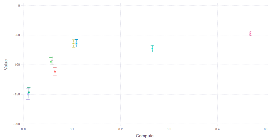
COMPUTE
Expected Cumulative Reward
Full POMDP (POMCPOW)
No Observations