Some Basic Statistical Tools
Notes
- Accessible reference for rigorous definitions of random variables, etc: Stanford STAT 219 Notes
- Example of a non-Borel set: Vitali set
Outline for Today
- Note on methods of learning
- Convergence for sequences of random variables
- Break
- Concentration inequalities
- Proof of the weak law of large numbers
- (If time) Proof techniques
Methods of Learning
(Disclaimer: I am not a trained epistemologist)
Testimony
Perception
(Scientific Method)
Reason
(Mathematical Proof)
- Read or hear a piece of knowledge
- Decide whether to believe it (e.g. based on authority of speaker)
- Learn by believing it
- Formulate a question
- Formulate a hypothesis
- Test the hypothesis with an experiment
- Learn by analyzing the results of the experiment
- Formulate a question
- Create a conjecture that answers the question
- Define all concepts
- State as a theorem
- Prove or disprove the conjecture
- Learn by considering the theorem/false conjecture and the proof
Most RL research fits into the scientific method.
Review
Given a probability space \((\Omega, \mathcal{F}, P)\), and a measurable space \((E, \mathcal{E})\), an \(E\)-valued random variable is a measurable function \(X: \Omega \to E\).
\(\omega \in \Omega\)
\(\Omega\)
\(\mathcal{F} = \sigma(\{\quad\}) = \{\Omega,\quad, \quad, \emptyset\}\)
\(\mathcal{F}\)
Review: Equality of Random Variables
Review: Convergence
For a (deterministic) sequence \(\{x_n\}\), we say
\[\lim_{n \to \infty} x_n = x\]
or
\[x_n \to x\]
if, for every \(\epsilon > 0\), there exists an \(N\) such that \(|x_n - x| < \epsilon\) for all \(n > N\).
Random Variables: Sure Convergence
\[X_n(\omega) \to X(\omega) \quad \forall \, \omega \in \Omega\]
Random Variables:
Almost Sure Convergence
\(X_n \stackrel{a.s.}{\to} X\) if and only if \(P(\{\omega: X_n(\omega) \to X\}) = 1\), that is, \(X_n\) converges to \(X\) except possibly on a zero-measure set.
Does sure convergence imply almost sure convergence?
Random Variables:
Convergence in Probability
\(X_n \to_p X\) if \(P(\{\omega : |X_n(\omega) - X(\omega) | > \epsilon\}) \to 0\) for any fixed \(\epsilon > 0\).
Does \(X_n \stackrel{a.s}{\to} X\) imply \(X_n \to_p X\)?
Does \(X_n \to_p X\) imply \(X_n \stackrel{a.s}{\to} X\)?
No.
But there exists a subsequence \(n_k\) such that \(X_{n_k} \stackrel{a.s.}{\to} X\).


Random Variables:
Convergence in Probability
Random Variables:
Weak Convergence
\(X_n \stackrel{D}{\to} X\) if \(F_{X_n}(\alpha) \to F_{X}(\alpha)\) for each fixed \(\alpha\) that is a continuity point of \(F_X\).
"Weak convergence", "convergence in distribution", and "convergence in law" all mean the same thing.
Summary
Convergence:
- Sure ("pointwise")
- Almost Sure
- In Probability
- Weak ("in distribution"/"in law")
\[X_n \to X \iff X_n(\omega) \to X(\omega) \quad \forall \, \omega \in \Omega\]
\[X_n \stackrel{a.s}{\to} X \iff P(\{\omega: X_n(\omega) \to X\}) = 1\]
\(X_n \to_p X \iff P(\{\omega : |X_n(\omega) - X(\omega) | > \epsilon\}) \to 0 \quad \forall \epsilon > 0\)
\(X_n \stackrel{D}{\to} X \iff F_{X_n}(\alpha) \to F_{X}(\alpha)\) for each continuity point.
Break: Convergence of MC integration
\[Q_N \to \frac{\pi}{4} \text{ (sure)?}\]
\[Q_N \stackrel{a.s.}{\to} \frac{\pi}{4} \text{?}\]
\[Q_N \to_p \frac{\pi}{4} \text{?}\]
\[Q_N \stackrel{D}{\to} \frac{\pi}{4} \text{?}\]

\[Q_N \equiv \frac{1}{N} \sum_{i=1}^{N} \mathbf{1}_{X_{i,1}^2 + X_{i,2}^2 \leq 1} (X_i)\]
\(X_i \sim U([0,1]^2)\)
(Intuitively)
Convergence of MC integration
\[Q_N \to \mu \text{ (sure)?}\]
\[Q_N \stackrel{a.s.}{\to} \mu \text{?}\]
\[Q_N \to_p \mu \text{?}\]
\[Q_N \stackrel{D}{\to} \mu \text{?}\]
\(\exists \omega \in \Omega\) where you always sample the same point.
Probability that there are enough measurements off in one direction to keep \(|Q_N - \mu| > \epsilon\) decays with more samples.
Weak law of large numbers
Strong law of large numbers
Concentration Inequalities
Concentration inequalities take the form
\[P(X \geq t) \leq \phi(t)\]
where \(\phi\) goes to zero (quickly) as \(t \to \infty\)
Intuition: If an r.v. has a finite variance, the probability that a random variable takes a value far from its mean should be small
Concentration Inequalities
Markov's Inequality:
If \(X \geq 0\), then \[P(X \geq t) \leq \frac{E[X]}{t}\quad \forall \, t \geq 0\]
Concentration Inequalities
Markov's Inequality:
If \(X \geq 0\), then \[P(X \geq t) \leq \frac{E[X]}{t}\quad \forall \, t \geq 0\]
Concentration Inequalities
Markov's Inequality:
If \(X \geq 0\), then \[P(X \geq t) \leq \frac{E[X]}{t}\quad \forall \, t \geq 0\]
General, but very loose
Concentration Inequalities
Chebyshev's Inequality:
Let \(X\) be any real-valued random variable with \(\text{Var}(X) < \infty\). Then
\[P(|X-E[X]| \geq t) \leq \frac{\text{Var}(X)}{t^2}\text{.}\]
Very general, but still loose
Concentration Inequalities
Chebyshev's Inequality:
Let \(X\) be any real-valued random variable with \(\text{Var}(X) < \infty\). Then
\[P(|X-E[X]| \geq t) \leq \frac{\text{Var}(X)}{t^2}\text{.}\]
Very general, but still loose
Concentration Inequalities
Chebyshev's Inequality
Concentration Inequalities
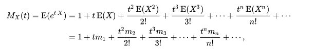
Moment generating function: \(M_X(t) \equiv E[e^{tX}]\)
Chernoff Bound: If the moment-generating function \(M_X\) exists, then
\[P(X \geq a) \leq \frac{E[e^{tX}]}{e^{ta}} \quad \forall\, t > 0\]
and
\[P(X \leq a) \leq \frac{E[e^{tX}]}{e^{ta}} \quad \forall\, t < 0\]
Tighter than Markov and Chebyshev
Bonus Slide: Moment Generating Functions
To get the \(n\)th moment from \(M_X(t)\), differentiate it \(n\) times and set \(t=0\).
Because:
Concentration Inequalities
Moment generating function: \(M_X(t) \equiv E[e^{tX}]\)
Chernoff Bound: If the moment-generating function \(M_X\) exists, then
\[P(X \geq a) \leq \frac{E[e^{tX}]}{e^{ta}} \quad \forall\, t > 0\]
and
\[P(X \leq a) \leq \frac{E[e^{tX}]}{e^{ta}} \quad \forall\, t < 0\]
Tighter than Markov and Chebyshev
Concentration Inequalities
Name
Requirements
Bound
Chebyshev
\(\text{Var}(X) < \infty\)
\[P(|X-E[X]| \geq t) \leq \frac{\text{Var}(X)}{t^2}\]
Markov
\(X\geq 0\), \(\text{E}[X]\) exists
\[P(X \geq t) \leq \frac{E[X]}{t}\quad \forall \, t \geq 0\]
Chernoff
\(M_X\) exists
\[P(X \geq a) \leq \frac{E[e^{tX}]}{e^{ta}} \quad \forall\, t > 0\]
\[P(X \leq a) \leq \frac{E[e^{tX}]}{e^{ta}} \quad \forall\, t < 0\]
Exercise
Let \(Y\) be a r.v. that takes values in \([-1,1]\) with mean -0.5. Give an upper bound on the probability that \(Y \geq 0.5\).
Name
Requirements
Bound
Chebyshev
\(\text{Var}(X) < \infty\)
\[P(|X-E[X]| \geq t) \leq \frac{\text{Var}(X)}{t^2}\]
Markov
\(X\geq 0\), \(\text{E}[X]\) exists
\[P(X \geq t) \leq \frac{E[X]}{t}\quad \forall \, t \geq 0\]
Chernoff
\(M_X\) exists
\[P(X \geq a) \leq \frac{E[e^{tX}]}{e^{ta}} \quad \forall\, t > 0\]
\[P(X \leq a) \leq \frac{E[e^{tX}]}{e^{ta}} \quad \forall\, t < 0\]
Break
Let \(Y\) be a r.v. that takes values in \([-1,1]\) with mean -0.5. Give an upper bound on the probability that \(Y \geq 0.5\).
Name
Requirements
Bound
Chebyshev
\(\text{Var}(X) < \infty\)
\[P(|X-E[X]| \geq t) \leq \frac{\text{Var}(X)}{t^2}\]
Markov
\(X\geq 0\), \(\text{E}[X]\) exists
\[P(X \geq t) \leq \frac{E[X]}{t}\quad \forall \, t \geq 0\]
Chernoff
\(M_X\) exists
\[P(X \geq a) \leq \frac{E[e^{tX}]}{e^{ta}} \quad \forall\, t > 0\]
\[P(X \leq a) \leq \frac{E[e^{tX}]}{e^{ta}} \quad \forall\, t < 0\]
(Weak) Law of large numbers
Let \(X_i\) be independent identically distributed r.v.s with mean \(\mu\) and variance \(\sigma^2\). If \(Q_N \equiv \frac{1}{N} \sum_{i=1}^N X_i\), then \(Q_N \to_p \mu\).
Proof:
(Weak) Law of large numbers
Let \(X_i\) be independent identically distributed r.v.s with mean \(\mu\) and variance \(\sigma^2\). If \(Q_N \equiv \frac{1}{N} \sum_{i=1}^N X_i\), then \(Q_N \to_p \mu\).
Proof:
Law of Large Numbers
Two somewhat astounding takeaways:
1. Standard deviation decays at \(\frac{1}{\sqrt{N}}\) regardless of dimension.
2. You can estimate the "standard error" with \[SE = \frac{s}{\sqrt{N}}\]
where \(s\) is the sample standard deviation.
Confidence Intervals
How do you estimate \(|Q_N - \mu|\)?
Given a random variable \(Q\), a \(\gamma\) Confidence Interval, \([u(Q), v(Q)]\), is a random interval that contains \(\mu\) with probability \(\gamma\), i.e. \[P(u(Q) \leq \mu \leq v(Q)) = \gamma\]
Example: \(Q_N \equiv \frac{1}{N} \sum_{i=1}^N X_i\)
Idea for approximate confidence interval: estimate \(\text{Var}(Q_N)\) with \(SE^2 = \frac{s^2}{N}\) and use Chebyshev.
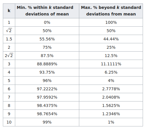
Confidence Intervals
Idea for approximate confidence interval: estimate \(\text{Var}(Q_N)\) with \(SE^2 = \frac{s^2}{N}\) and use Chebyshev.
\[P(| X - E[X] | \geq t) \leq \frac{\text{Var}(X)}{t^2} = 1-\gamma = 0.05\]
Use \(\gamma = 0.95\)
\[t = \sqrt{\frac{\text{Var}(X)}{0.05}}\]
\[t \approx \frac{SE}{\sqrt{0.05}} \approx 4.47 SE\]
Approximate 95% CI: \([Q_N - 4.47\,SE, Q_N + 4.47 \,SE]\)
We can do much better if we know something about the distribution of \(Q_N\)!
Central Limit Theorem
Lindeberg-Levy CLT: If \(\text{Var}[X_i] = \sigma^2 < \infty\), then
\[\sqrt{N}(Q_N - \mu) \stackrel{D}{\to} \mathcal{N}(0, \sigma)\]
After many samples \(Q_N\) starts to look distributed like \(\mathcal{N}(\mu, \frac{\sigma}{\sqrt{N}})\)
\(Q_1 \overset{D}{=} X_i\)
Confidence Intervals
Idea for approximate confidence interval: estimate \(\text{Var}(Q_N)\) with \(SE^2 = \frac{s^2}{N}\) and use Chebyshev the central limit theorem.
For a normal distribution,
\[P(|X-\mu| \geq t) = 1+ \text{erf}\left(\frac{t-\mu}{\sqrt{2} \sigma}\right)\]
Use \(\gamma = 0.95\)
Approximate 95% CI: \([Q_N - 1.96\,SE, Q_N + 1.96 \,SE]\)
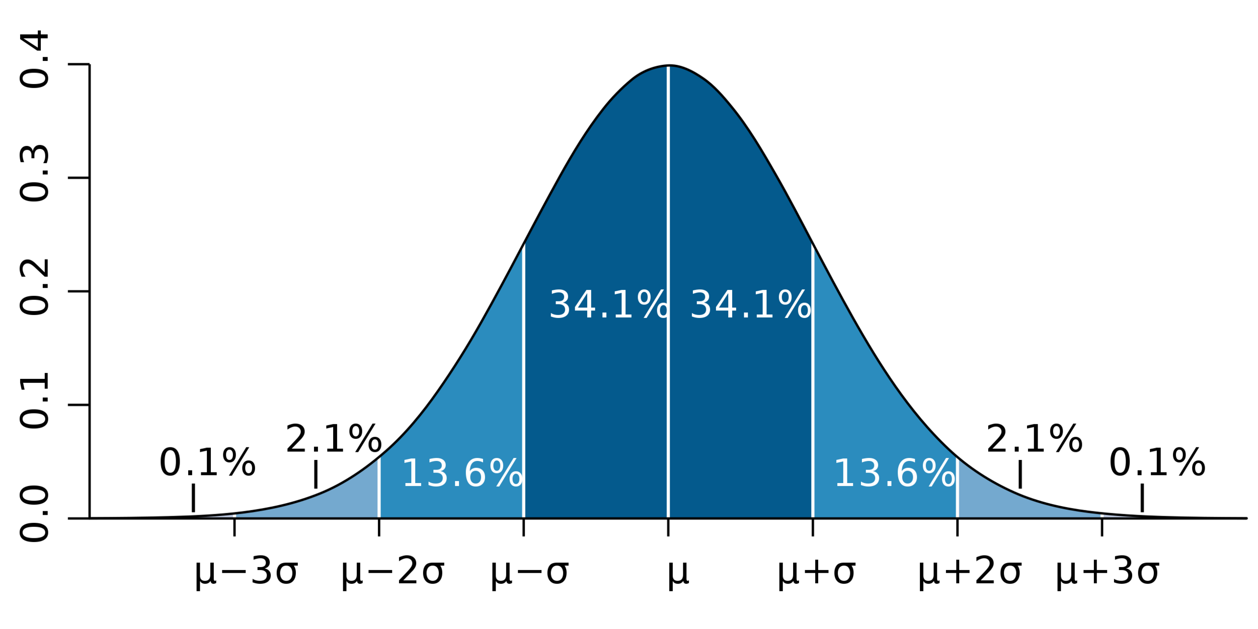
(Chebyshev gave 4.47)
\(t \approx 1.96 SE\)
Importance Sampling
\[E[X] = \int x \, p(x)\, dx\]
\[=\int x \, \frac{p(x)}{q(x)}q(x) \, dx\]
\[\approx \frac{1}{N} \sum Y_i \frac{p(Y_i)}{q(Y_i)}\]
\[\approx \frac{1}{N} \sum Y_i w_i\] where \(w_i = \frac{p(Y_i)}{q(Y_i)}\)
Want to estimate \(X \sim p\) with samples from \(Y_i \sim q\).
Summary
- Concentration Inequalities
- Law of large numbers
- Central Limit Theorem
- Importance Sampling
\(Q_N \to_p \mu\)
\(Q_N \stackrel{D}{\to} \mathcal{N}(\mu, \frac{\sigma}{\sqrt{N}})\)
\[P(X \geq t) \leq \phi(t)\]
\[E[X]\approx \frac{1}{N} \sum Y_i w_i\] where \(w_i = \frac{p(Y_i)}{q(Y_i)}\)