Autonomous Navigation Among Dynamic Obstacles
Himanshu Gupta
Masters Student, Computer Science, University of Colorado Boulder


Autonomous systems in the real world

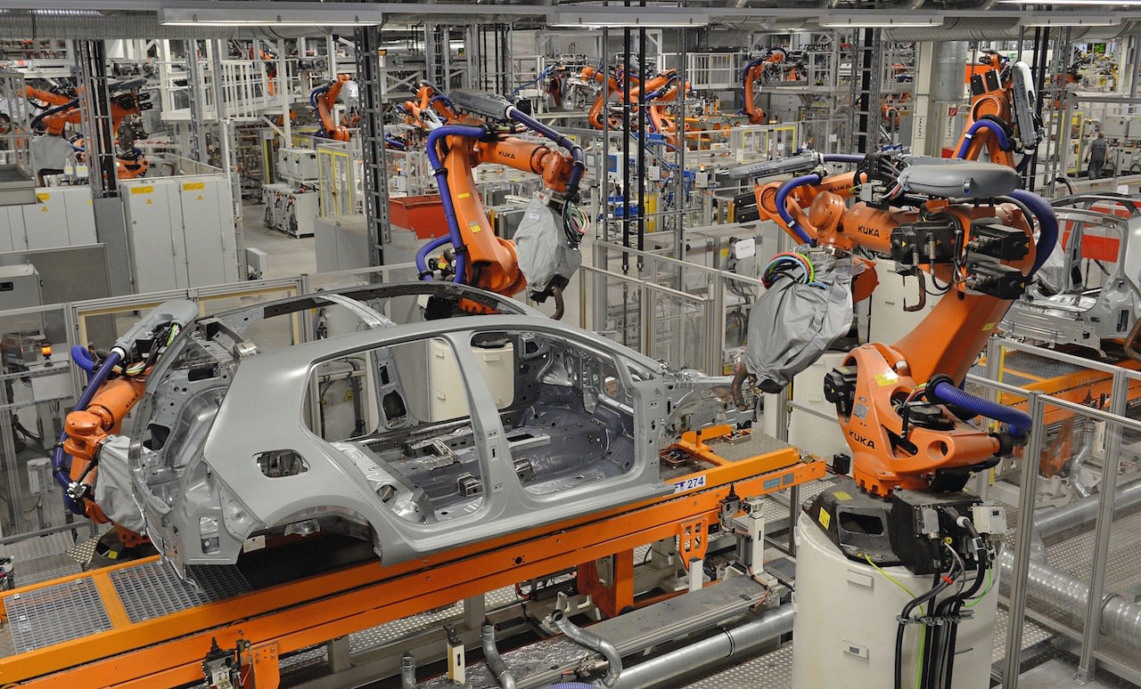

Autonomous Navigation among dense Crowds of Pedestrians and Obstacles
Prior Work
Pedestrian Modeling
- Use recorded trajectories to learn pedestrian dynamics.
(Alahi et. al, CVPR 16; Chen et. al, GNCC 16)
- Pedestrian motion model that accounts for both intentions and interactions (Luo et. al, IRAL 18)

Prior Work
Reactive Controllers
- Fox et. al, IARM 97
- Schiller et. al, ISIV 98


Issues
- Pedestrian Model?
- Future effect of imemdiate actions?
Prior Work
Predict and act
controllers
- Kuwata et. al, TCST 09
- Berg et. al, IJRR 11


Issues
- Uncertainty in pedestrian intention estimation?
Two major questions
-
How to reason over uncertainty in pedestrian intention estimation?
- How to determine the optimal action for the vehicle at any given point of time with arbitrary uncertainty?
POMDP
- A mathematical framework for optimal decision-making in the presence of various types of uncertainty!

Contributions
-
We propose a new technique for navigation problems with arbitrary state uncertainty by incorporating multi-query path planning techniques for effective tree search using online solvers for a POMDP
- Probabilistic RoadMaps
-
Fast Marching Methods
- Demonstrate that our technique outperforms the current state-of-the-art method significantly in terms of travel time while being just as safe!
Preliminaries
Types of Uncertainty
OUTCOME
MODEL
STATE


Markov Model
- \(\mathcal{S}\) - State space
- \(T:\mathcal{S}\times\mathcal{S} \to \mathbb{R}\) - Transition probability distributions
Markov Decision Process (MDP)
- \(\mathcal{S}\) - State space
- \(T:\mathcal{S}\times \mathcal{A} \times\mathcal{S} \to \mathbb{R}\) - Transition probability distribution
- \(\mathcal{A}\) - Action space
- \(R:\mathcal{S}\times \mathcal{A} \to \mathbb{R}\) - Reward

Solving MDPs - The Value Function
$$V^*(s) = \underset{a\in\mathcal{A}}{\max} \left\{R(s, a) + \gamma E\Big[V^*\left(s_{t+1}\right) \mid s_t=s, a_t=a\Big]\right\}$$
Involves all future time
Involves only \(t\) and \(t+1\)
$$\underset{\pi:\, \mathcal{S}\to\mathcal{A}}{\mathop{\text{maximize}}} \, V^\pi(s) = E\left[\sum_{t=0}^{\infty} \gamma^t R(s_t, \pi(s_t)) \bigm| s_0 = s \right]$$
$$Q(s,a) = R(s, a) + \gamma E\Big[V^* (s_{t+1}) \mid s_t = s, a_t=a\Big]$$
Value = expected sum of future rewards
Online Decision Process Tree Approaches

Time
Estimate \(Q(s, a)\) based on children
$$Q(s,a) = R(s, a) + \gamma E\Big[V^* (s_{t+1}) \mid s_t = s, a_t=a\Big]$$
\[V(s) = \max_a Q(s,a)\]
Partially Observable Markov Decision Process (POMDP)

- \(\mathcal{S}\) - State space
- \(T:\mathcal{S}\times \mathcal{A} \times\mathcal{S} \to \mathbb{R}\) - Transition probability distribution
- \(\mathcal{A}\) - Action space
- \(R:\mathcal{S}\times \mathcal{A} \to \mathbb{R}\) - Reward
- \(\mathcal{O}\) - Observation space
- \(Z:\mathcal{S} \times \mathcal{A}\times \mathcal{S} \times \mathcal{O} \to \mathbb{R}\) - Observation probability distribution

State
Timestep
Accurate Observations
Goal: \(a=0\) at \(s=0\)
Optimal Policy
Localize
\(a=0\)
POMDP Example: Light-Dark
POMDP Sense-Plan-Act Loop
Environment
Belief Updater
Policy
\(b\)
\(a\)
\[b_t(s) = P\left(s_t = s \mid a_1, o_1 \ldots a_{t-1}, o_{t-1}\right)\]

True State
\(s = 7\)
Observation \(o = -0.21\)
Solving a POMDP
- Obtaining exact solutions to POMDPs is an intractable problem [1].
- They are solved approximately in an online fashion by performing a tree search over the belief space.
[1] Christos H. Papadimitriou and John N. Tsitsiklis. 1987. The Complexity of Markov Decision Processes. Mathematics of Operations Research 12, 3 (1987), 441–450.

Action Nodes
Belief Nodes
- A POMDP is an MDP on the Belief Space but belief updates are expensive.
-
POMCP* uses simulations of histories instead of full belief updates
- Each belief is implicitly represented by a collection of either unweighted or weighted particles

[Ross, 2008] [Silver, 2010]
*(Partially Observable Monte Carlo Planning)
Solving a POMDP
Solving a POMDP


Roll-out Policy is important
Solving a POMDP using DESPOT
- Tree search in DESPOT is guided by a lower bound and an upper bound on the value estimates at each belief node.
- The lower bound is generally obtained by executing a roll-out policy.
- The upper bound can be obtained by overestimation.
Roll-out Policy is important
Technical Work
Bai et. al's Approach

\(1D\)-\(A^*\)
\(1D-A^*\) Approach

Hybrid \(A^*\) Path Planning
-
Hybrid \(𝐴^∗\) is an extension of \(𝐴^∗\) for continuous state space.
- It finds the trajectory with minimum cost from the vehicle’s current position to its goal location.
\(\rho = [(x_0,y_0), (x_1,y_1).....(x_n,y_n))]\)
$$ C(\rho) = \sum_{i=0}^{n} ( \lambda^i C_{st}(x_i, y_i) + \lambda^i C_{ped}(x_i, y_i)) $$
\(1D-A^*\) Approach
\(1D-A^*\) Approach
POMDP Model for \(1D\)-\(A^*\) Approach
-
STATE Modeling: ( Vehicle state, Vector of \(n_{ped}\) nearby pedestrian states)
- Vehicle state: \((x_c(t),y_c(t),\theta_c(t),v_c(t))\)
- \(i^{th}\) pedestrian's state: \((x_i(t),y_i(t),v_i(t), g_i)\)
$$\mathcal{s(t)} = (x_c(t), y_c(t), \theta_c(t), v_c(t), [ (x_1(t), y_1(t), v_1(t), g_1), \\ (x_2(t), y_2(t), v_2(t), g_2),...,(x_{n_{ped}}(t), y_{n_{ped}}(t), v_{n_{ped}}(t), g_{n_{ped}})])$$
POMDP Model for \(1D\)-\(A^*\) Approach
-
ACTION Modeling:
Change in vehicle speed along the Hybrid \(A^*\) path
$$\delta_s(t) \in \{\textbf{Increase Speed, Decrease Speed,}$$ $$\textbf{Maintain Speed, Sudden Brake\}}$$
POMDP Model for \(1D\)-\(A^*\) Approach
-
OBSERVATION Modeling:
(Vehicle position, Vector of discretized positions of the \(n_{ped}\) nearby pedestrians)
$$\mathcal{o(t)} = (x_c(t), y_c(t), [ (x_1'(t), y_1'(t)), (x_2'(t), y_2'(t)),...,(x_{n_{ped}}'(t), y_{n_{ped}}'(t))])$$
POMDP Model for \(1D\)-\(A^*\) Approach
-
REWARD Modeling:
- Goal reward \(R_{goal}\)
- Pedestrian Collision Penalty \(R_{ped}\)
- Low speed penalty \(R_{speed}\)
- Sudden Break penalty \(R_{SB}\)
-
\(R_{t}\)
- BELIEF: - A joint probability distribution over goals for all \(n_{ped}\) pedestrians
POMDP Model for \(1D\)-\(A^*\) Approach
-
GENERATIVE FUNCTION:
Applies action \(a\) to state \(s\) and obtain the new state \(s'\), immediate reward \(r\) and observation \(o\).
$$G(s,a) = (s',r,o)$$
Solving POMDP using DESPOT
- Perform tree search using forward simulations with the generative function \(G\).
- Lower bound for a leaf belief node
- Execute a rollout policy
- Reactive controller over the generated hybrid \(A^*\) path
- Reactive controller over the generated hybrid \(A^*\) path
- Execute a rollout policy
- Upper bound for a leaf belief node
- \(R_{ped}\)
- \(\gamma^t R_{goal}\)
\(1D-A^*\) Approach
\(\textbf{1D-A}^*\) Approach

\(\textbf{1D-A}^*\) Approach - Drawbacks
- Decoupling of heading angle planning and speed planning often leads to unnecessary stalling of the vehicle!
- Hybrid A* path can't be found at at every time step!
2D - Approach

2D Approach

POMDP Model for \(2D\) approach
-
STATE Modeling: ( Vehicle state, Vector of \(n_{ped}\) nearby pedestrian state)
- Vehicle state: \((x_c(t),y_c(t),\theta_c(t),v_c(t))\)
- \(i^{th}\) pedestrian's state: \((x_i(t),y_i(t),v_i(t), g_i)\)
$$\mathcal{s(t)} = (x_c(t), y_c(t), \theta_c(t), v_c(t), [ (x_1(t), y_1(t), v_1(t), g_1), \\ (x_2(t), y_2(t), v_2(t), g_2),...,(x_{n_{ped}}(t), y_{n_{ped}}(t), v_{n_{ped}}(t), g_{n_{ped}})])$$
POMDP Model for \(2D\) approach
-
ACTION Modeling:
( Change in vehicle's heading angle, Change in vehicle's speed)
$$\mathcal{a = ( \delta_\theta(t) , \delta_s(t) )}$$
POMDP Model for \(2D\) approach
-
OBSERVATION Modeling:
(Vehicle position, Vector of discretized positions of the \(n_{ped}\) nearby pedestrians)
$$\mathcal{o(t)} = (x_c(t), y_c(t), [ (x_1'(t), y_1'(t)), (x_2'(t), y_2'(t)),...,(x_{n_{ped}}'(t), y_{n_{ped}}'(t))])$$
POMDP Model for \(2D\) approach
-
REWARD Modeling:
- Goal reward \(R_{goal}\)
- Static Obstacle Collision Penalty \(R_{obs}\)
- Pedestrian Collision Penalty \(R_{ped}\)
- Low speed penalty \(R_{speed}\)
- Sudden stop penalty \(R_{SB}\)
-
\(R_{t}\)
- BELIEF: - A joint probability distribution over goals for all \(n_{ped}\) pedestrians
POMDP Model for \(2D\) approach
-
GENERATIVE FUNCTION:
Applies action \(a\) to state \(s\) and obtain the new state \(s'\), immediate reward \(r\) and observation \(o\).
$$G(s,a) = (s',r,o)$$
Solving POMDP using DESPOT
- Perform tree search using forward simulations with the generative function \(G\).
- Lower bound for a leaf belief node
- Execute a rollout policy
- Execute a rollout policy
- Upper bound for a leaf belief node
- \(R_{ped}\)
- \(\gamma^t R_{goal}\)
2D Approach
2D Approach - Issues
- An expansion of the action space opens up a much larger region of the state space to exploration.
- Critical Challenge: Determining a good roll-out policy for the vastly increased set of states reachable in the tree search.
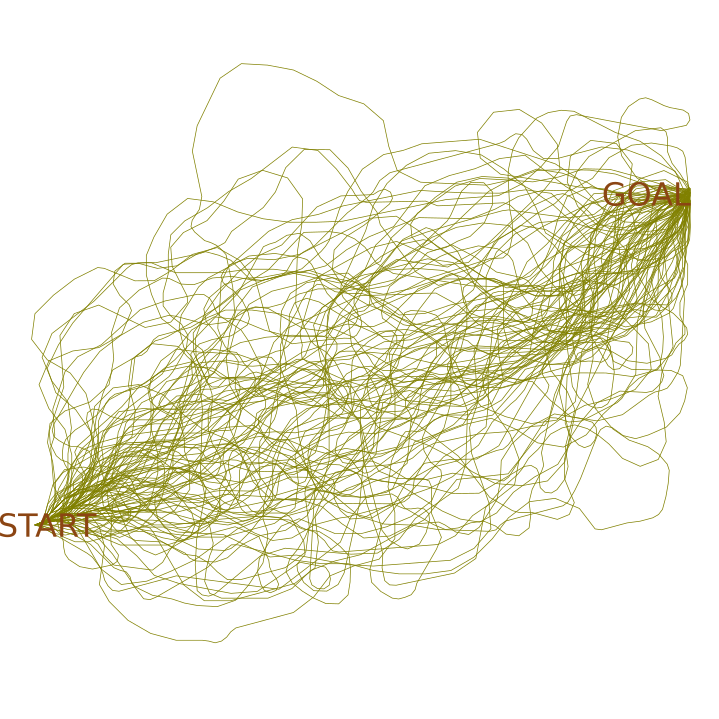
Generating Effective Rollout Policy
-
An effective rollout policy
-
Execute a path from the vehicle's current position to its goal location
-
-
Rely on Multi-query Path Planning Techniques
-
Probabilistic RoadMaps
-
Fast Marching Method
-
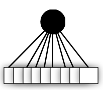
Probabilistic RoadMaps for Multi-Query Path Planning
-
The Probabilistic Roadmap or 𝑃𝑅𝑀 is a method for path planning in high dimensions for robots in static environments.
Probabilistic RoadMaps for Multi-Query Path Planning

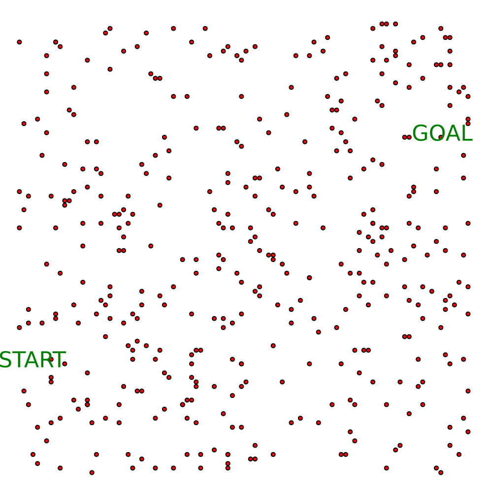
Fast Marching Method for Multi-Query Path Planning
-
The Fast Marching Method (𝐹𝑀𝑀) is an algorithm for tracking and modeling the motion of a physical wave interface.
-
𝐹𝑀𝑀 calculates the time that the wave takes to reach all points in the environment.
Fast Marching Method for Multi-Query Path Planning

G
Fast Marching Method for Multi-Query Path Planning
G


2D Approach

\(2D-FMM\)
2D Approach
Experiments
Experiments
- Simulation environment
- Experimental scenarios
- Different planners
- Experimental details
Simulation Environment
- Environment: \(100\)m x \(100\)m square field

-
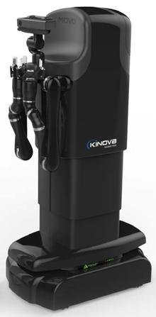
Autonomous vehicle: A holonomic vehicle.
- Inspired by Kinova MOVO
- Max speed: \(2\) m/s
Simulation Environment
- Pedestrians are assigned one of the four goals at randon

Experimental Scenarios
Scenario 1
(Open Field)
Experimental Scenarios

Scenario 2 (Cafeteria Setting)
Experimental Scenarios
Scenario 3
(L shaped lobby)

Experimental Scenarios
Scenario 1
(Open Field)
Scenario 2 (Cafeteria Setting)
Scenario 3
(L shaped lobby)
Planners
Limited Space
Planner
Extended Space
Planners
\(1D\)-\(A^*\)
\(2D\)-\(PRM\)
\(2D\)-\(FMM\)
Planners
-
Hybrid \(A^*\) Path Planning (36 options)
$$\delta_{\theta}\in \{-170 \degree, -160 \degree,..., -10 \degree, 0 \degree, 10\degree,....170\degree, 180\degree \}$$ -
POMDP Speed Planning (4 options)
$$\delta_s\in \{-1 \textbf{m/s}, 0 \textbf{m/s}, 1 \textbf{m/s}, \textbf{Sudden Brake} \}$$
- Roll-out policy for lower bound: Reactive controller over the generated \(A^*\) path
\(1D\)-\(A^*\)
Planners
\(2D\)-\(PRM\)
-
POMDP Heading and Speed Planning \((\delta_{\theta},\delta_s)\)
-
When \(v_c = 0\) ( 9 choices)
- Stay Stationary \((0 \degree,0 \textbf{m/s})\)
- Move \((-45 \degree,1 \textbf{m/s})\), \((-30 \degree,1 \textbf{m/s})\), \((-15 \degree,1 \textbf{m/s})\), \((0 \degree,1 \textbf{m/s})\), \((15 \degree,1 \textbf{m/s})\), \((30 \degree,1 \textbf{m/s})\), \((45 \degree,1 \textbf{m/s})\), \((\delta_{RO},1 \textbf{m/s})\)
-
When \(v_c \neq 0\) ( 11 choices)
- Maintain heading and speed \((0 \degree,0 \textbf{m/s})\)
- Maintain heading but change speed \((0 \degree,1 \textbf{m/s})\), \((0 \degree,-1 \textbf{m/s})\)
- Maintain speed but modify heading \((-45 \degree,0 \textbf{m/s})\), \((-30 \degree,0 \textbf{m/s})\), \((-15 \degree,0 \textbf{m/s})\), \((15 \degree,0 \textbf{m/s})\), \((30 \degree,0 \textbf{m/s})\), \((45 \degree,0 \textbf{m/s})\), \((\delta_{RO},0 \textbf{m/s})\)
- Apply Sudden Break \((0 \degree, \textbf{SB})\)
-
When \(v_c = 0\) ( 9 choices)
Planners
\(2D\)-\(PRM\)
- Roll-out policy for lower bound: Reactive controller over the obtained PRM path
Planners
-
POMDP Heading and Speed Planning \((\delta_{\theta},\delta_s)\)
-
When \(v_c = 0\) ( 9 choices)
- Stay Stationary \((0 \degree,0 \textbf{m/s})\)
- Move \((-45 \degree,1 \textbf{m/s})\), \((-30 \degree,1 \textbf{m/s})\), \((-15 \degree,1 \textbf{m/s})\), \((0 \degree,1 \textbf{m/s})\), \((15 \degree,1 \textbf{m/s})\), \((30 \degree,1 \textbf{m/s})\), \((45 \degree,1 \textbf{m/s})\), \((\delta_{RO},1 \textbf{m/s})\)
-
When \(v_c \neq 0\) ( 11 choices)
- Maintain heading and speed \((0 \degree,0 \textbf{m/s})\)
- Maintain heading but change speed \((0 \degree,1 \textbf{m/s})\), \((0 \degree,-1 \textbf{m/s})\)
- Maintain speed but modify heading \((-45 \degree,0 \textbf{m/s})\), \((-30 \degree,0 \textbf{m/s})\), \((-15 \degree,0 \textbf{m/s})\), \((15 \degree,0 \textbf{m/s})\), \((30 \degree,0 \textbf{m/s})\), \((45 \degree,0 \textbf{m/s})\), \((\delta_{RO},0 \textbf{m/s})\)
- Apply Sudden Break \((0 \degree, \textbf{SB})\)
-
When \(v_c = 0\) ( 9 choices)
\(2D\)-\(FMM\)
Planners
\(2D\)-\(FMM\)
- Roll-out policy for lower bound: Reactive controller over the obtained FMM path
Experimental Details
- For each scenario, we ran sets of 100 different experiments with different pedestrian densities in the environment.
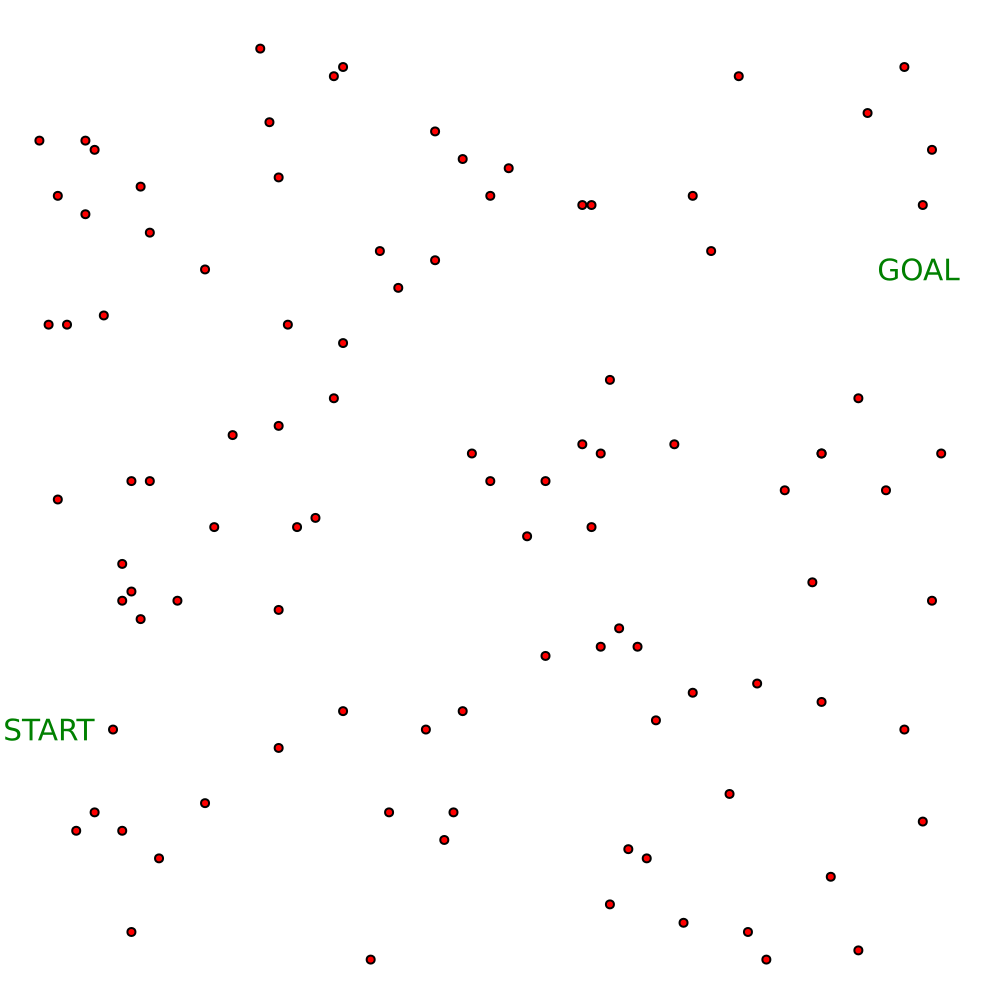


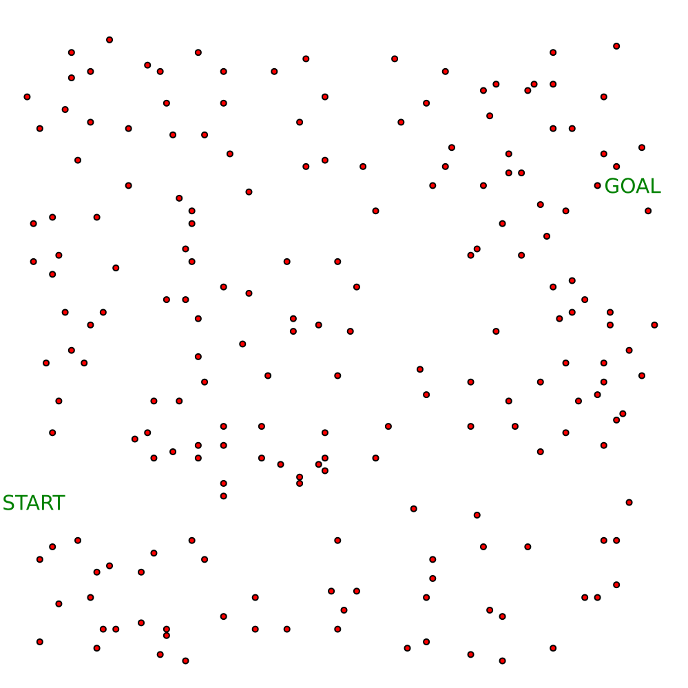
# humans = 100
# humans = 200
# humans = 300
# humans = 400
Scenario 1
Experimental Details
- In simulations, the planning time for the vehicle at each step is 0.5 seconds

Experimental Details
- The performance of different planners was compared for a sampled environment under the same random seed for noise in simulated pedestrian motion.
Results (HV)
Evaluation Metrics:
- Travel Time (in s)
- #SB actions
- #Outperformed
Results (HV)
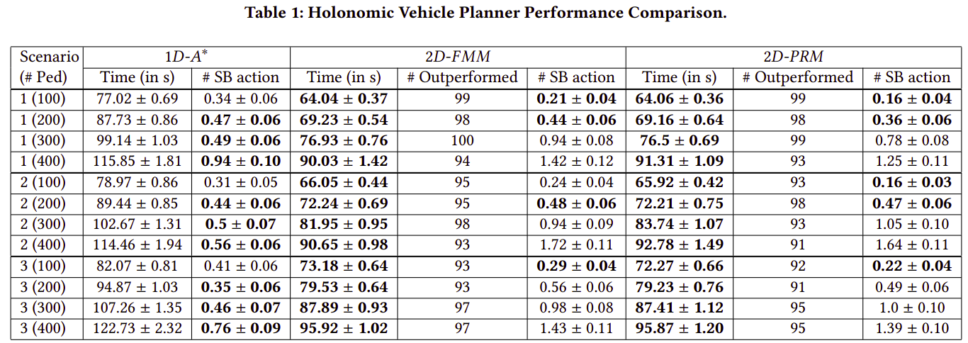
Evaluation Metric: Travel Time (in s)
Results (HV)
Evaluation Metric: #Outperformed
Results (HV)


Scenario 1
\(1D-A^*\)
\(2D-FMM\)
\(2D-PRM\)
Results (HV)
Scenario 2


\(1D-A^*\)
\(2D-FMM\)
\(2D-PRM\)
Results (HV)
Scenario 3


\(1D-A^*\)
\(2D-FMM\)
\(2D-PRM\)
Results (HV)
Evaluation Metric: #SB action
Experiments (NHV)
Simulation Environment
- Environment: \(100\)m x \(100\)m square field
-
Autonomous vehicle: A non- holonomic vehicle.
- Inspired by Dubin's car
- Max speed: \(4\) m/s

Experimental Scenario
Planners (NHV)
Limited Space
Planner
Extended Space
Planners
\(1D\)-\(A^*\)
\(2D\)-\(NHV\)
Planners (NHV)
-
Hybrid \(A^*\) Path Planning (19 options)
$$\delta_{\theta}\in \{-45 \degree, -40 \degree,..., -5 \degree, 0 \degree, 5\degree,....40\degree, 45\degree \}$$ -
POMDP Speed Planning (4 options)
$$\delta_s\in \{-1 \textbf{m/s}, 0 \textbf{m/s}, 1 \textbf{m/s}, \textbf{Sudden Brake} \}$$
- Roll-out policy for lower bound: Reactive Controller over the generated \(A^*\) path
\(1D\)-\(A^*\)
Planners
-
POMDP Heading and Speed Planning \((\delta_{\theta},\delta_s)\)
-
When \(v_c = 0\) ( 9 choices)
- Stay Stationary \((0 \degree,0 \textbf{m/s})\)
- Move \((-45 \degree,1 \textbf{m/s})\), \((-30 \degree,1 \textbf{m/s})\), \((-15 \degree,1 \textbf{m/s})\), \((0 \degree,1 \textbf{m/s})\), \((15 \degree,1 \textbf{m/s})\), \((30 \degree,1 \textbf{m/s})\), \((45 \degree,1 \textbf{m/s})\), \((\delta_{RO},1 \textbf{m/s})\)
-
When \(v_c \neq 0\) ( 11 choices)
- Maintain heading and speed \((0 \degree,0 \textbf{m/s})\)
- Maintain heading but change speed \((0 \degree,1 \textbf{m/s})\), \((0 \degree,-1 \textbf{m/s})\)
- Maintain speed but modify heading \((-45 \degree,0 \textbf{m/s})\), \((-30 \degree,0 \textbf{m/s})\), \((-15 \degree,0 \textbf{m/s})\), \((15 \degree,0 \textbf{m/s})\), \((30 \degree,0 \textbf{m/s})\), \((45 \degree,0 \textbf{m/s})\), \((\delta_{RO},0 \textbf{m/s})\)
- Apply Sudden Break \((0 \degree, \textbf{SB})\)
-
When \(v_c = 0\) ( 9 choices)
\(2D\)-\(NHV\)
Planners (NHV)
\(2D\)-\(NHV\)
-
Roll-out policy for lower bound: Reactive controller over a straight-line path to the goal.
- Apply steering angle within the kinematic constraints
- Doesn't work for previously defined Scenario 2 and Scenario 3
Results (NHV)

Evaluation Metric: Travel Time (in s)
Results (NHV)
Evaluation Metric: #SB action
Results (NHV)
Evaluation Metric: #Outperformed
Results (NHV)

\(1D-A^*\)
\(2D-NHV\)
\(1D-A^*\)
\(2D-NHV\)
Conclusion
Future Work
- Extending this work for NHV using Hamilton Jacobi Bellman problem formulation.

Future Work
- Extending this work to a high DOF agent

- Robotic manipulator
(Pellegrinelli et. al, IROS 16)
Future Work
- Goal-Object Data Association for Life Long Learning

Future Work
- Continuous space POMDP solvers